Introduction to Probability - Part 2

• Maximum Likelihood Estimation
  • Likelihood
  • General MLE
  • MLE for Gaussian Distribution
• Naive Bayes classification
  • Naive Bayes classifier
  • Gaussian naive Bayes
  • Multinomial naive Bayes
  • Bernoulli naive Bayes
• Information Theory
  • Information of an event
  • Shannon Entropy
  • Cross-Entropy Estimation
  • Kullback–Leibler Divergence
  • Bonus: Wasserstein Distance
• References

In this section, by default, all random variables and distributions are considered to be discrete to fit with the Machine Learning aspect, where the input \(x\), predicted output \(y\), and the target value \(\hat y\), are discrete random variables. The involvement of any continuous random variable or distribution will be noted for specific cases.

---

Maximum Likelihood Estimation

Likelihood

The likelihood function (often simply called the likelihood) describes the joint probability of the observed data as a function of the parameters of the chosen statistical model. The likelihood of parameter \(\theta\) given data \(X\) is \(P(X\mid \ \theta)\), it is also often written as \(L(\theta \mid \ X)\)

• In other words, given a specific value for parameter \(\theta\) as the initial condition, the likelihood \(L(\theta \mid \ X)\) is the probability that we would observe the outcomes represented by data \(X\) by the distribution function \(P(X\mid \ \theta)\)

Given a sample of \(n\) independent and identically distribution (i.i.d.) random variable \(X_1, \cdots , \ X_n\) from some distribution function \(P(X \mid \ \theta)\). With a specific parameter \(\theta^*\), the likelihood can be calculated by:

\[\begin{equation} \begin{aligned} L(\theta\mid X_1, \cdots, X_n) &= P(X_1,\cdots,X_n\mid \ \theta)\\ &= \prod_{i=1}^nP(X_i\mid \ \theta) \end{aligned} \end{equation}\]

Example:

• Consider a coin flip task, we already know that the probability of having a head is \(p_H = 0.5\) for a perfectly fair coin. Flipping a fair coin twice, we have the likelihood of having two heads with the parameter \(\theta = p_H = 0.5\) is:

  \[P(HH\mid p_H = 0.5) = 0.5^2 = 0.25\]

• On the other hand, assume that this is not a fair coin and the probability of having a head is \(p_H = 0.4\), then the likelihood of having two heads is:

  \[P(HH\mid p_H = 0.4) = 0.4^2 = 0.16\]

The likelihood function is differently defined for discrete and continuous probability distributions, including:

• Discrete probability distribution:

  Let \(X\) be a discrete random variable with the PMF \(p\) depending on parameter \(\theta\). Then the function

  \[L(\theta \mid \ x) = p_\theta(x) = P_\theta(X = x)\]

  is considered as a function for \(\theta\), is the likelihood function, given the outcome \(x\) of the r.v. \(X\).

• Continuous probability distribution:

  Let \(X\) be a continuous random variable with the PDF \(f\) depending on parameter \(\theta\). Then the function

  \[L(\theta \mid \ x) = f_\theta(x)\]

  is considered as a function for \(\theta\), is the likelihood function, given the outcome \(x\) of the r.v. \(X\).

General MLE

Given data \(X = \{ x_1, \ x_2, \cdots, \ x_n\}\) with individual \(x_i\) is the independent event data point (\(X\) follows the i.i.d). Assume that \(X\) follows some kind of probability distribution \(p(.\mid \theta)\) with \(\theta\) as the parameter. To find the appropriate \(\theta_*\) value that the distribution can describe best \(X\), we can use Maximum Likelihood Estimation (MLE) to find the value of \(\theta_*\) so the following probability can be maximum:

\[\begin{equation} \begin{aligned} \theta_* &= \underset{\theta}{\operatorname{argmax}}\ p(x_1, \ x_2, \cdots, x_n\mid \theta) \\ &= \underset{\theta}{\operatorname{argmax}}\prod_{i=1}^np(x_i\mid \theta) \end{aligned} \end{equation}\]

• Intuition:
  • Let’s say \(p(x_i\mid \theta)\) is the probability of having \(x_i\) given \(\theta\). Then, \(p(x_1, \ x_2, \cdots, x_n\mid \theta)\) is the probability that all events \(x_1, \ x_2, \cdots, x_n\) happen at the same time on the conditional of \(\theta\). This is called the likelihood. MLE is to find parameter \(\theta\) to maximize the likelihood.

  • Moreover, assuming that each data point \(x_i\) is independent, we can approximate the likelihood by:

    \[\begin{aligned} p(x_1, \ x_2, \cdots, x_n\mid \theta) \approx \prod_{i=1}^np(x_i\mid \theta) \end{aligned}\]

To optimize an objective function, we have to find the partial derivative of individual parameters in terms of the objective function. However, it is more difficult and complex to find the derivative of a product than a sum. Therefore, instead of optimizing an objective function, we usually optimize the log of that function instead.

• Intuition:

  • \(\log\) of a product is equal to the sum of individual \(\log\):

    \[\log(a \cdot b) = \log(a) + \log(b)\]

  • \(\log\) is an monotonic function, therefore the maximum of \(f(.\mid \theta)\) occur at the same value of \(\theta\) as does the maximum of \(\log[f(.\mid \theta)]\), thus:

    \[\underset{\theta}{\operatorname{argmax}}\ f(x\mid \theta) = \underset{\theta}{\operatorname{argmax}}\ \log\left[f(x\mid \theta)\right]\]

  • In computer science and machine learning scope, by default, \(\log = \ln = \log_2\) (rather than \(\log_{10}\))

Therefore, the Maximum Likelihood Estimation problem will be converted to the Maximum Log-likelihood, which also be the main formula of Maximum Likelihood Estimation, to find the optimum \(\theta_*\) value:

\[\begin{equation} \theta_* = \underset{\theta}{\operatorname{argmax}}\sum_{i=1}^n \log[p(x_i\mid \theta)] \end{equation}\]

MLE for Gaussian Distribution

Given \(X = \{ x_1, \ x_2, \cdots, \ x_n\}\), an independent, identically distributed random variable that follows the Gaussian Distribution, with \(x_i\) as an independent data point, to estimate the two parameters \(\mu, \ \sigma\) we apply the Gaussian distribution function to the Maximum Likelihood formula, we have:

\[\begin{aligned} \mu, \ \sigma^2 &= \underset{\mu, \sigma^2}{\operatorname{argmax}} \prod_{n=1}^Np(x^n\mid \mu, \sigma^2)\\ &= \underset{\mu,\ \sigma^2}{\operatorname{argmax}}\left[\prod_{i=1}^n\frac{1}{\sqrt{2\pi\sigma^2}}\exp\left(- \frac{(x_i - \mu)^2}{2\sigma^2}\right) \right] \\&= \underset{\mu,\ \sigma^2}{\operatorname{argmax}}\left[\frac{1}{(2\pi\sigma^2)^\frac{n}{2}}\exp\left(- \frac{\sum_{i=1}^n(x_i - \mu)^2}{2\sigma^2}\right) \right] \end{aligned}\]

By applying the \(\log\) function, we have:

\[\begin{aligned} \mu,\ \sigma^2 &= \underset{\mu,\ \sigma^2}{\operatorname{argmax}}\left(-\frac{n}{2}\log(2\pi) - n\log(\sigma) - \frac{\sum_{i=1}^n(x_i - \mu)^2}{2\sigma^2} \right) \\ &\triangleq \underset{\mu,\ \sigma^2}{\operatorname{argmax}} \ J(\mu,\ \sigma) \end{aligned}\]

• We can remove \(-\frac{n}{2}\log(2\pi)\) as it is a constant value that does not affect the calculation

To find the optimal \(\mu\) and \(\sigma\), we need to calculate the partial derivative of \(J(\mu,\ \sigma)\) on two parameters when they equal to 0 by:

\[\begin{aligned} \frac{\partial J}{\partial \mu} = \frac{1}{\sigma^2}\sum_{i=1}^n(x_i - \mu) = 0 \quad &\Rightarrow \quad \mu = \frac{1}{n}\sum_{i=1}^nx_i \\ \frac{\partial J}{\partial \sigma} = -\frac{n}{\sigma} + \frac{1}{\sigma^3}\sum_{i=1}^n(x_i - \mu)^2 = 0 \quad &\Rightarrow \quad \sigma^2 = \frac{1}{n}\sum_{i=1}^n(x_i - \mu)^2 \end{aligned}\]

As you can see, the obtained formula of \(\mu\) and \(\sigma\) are two formulas that we usually use to find the expectation and variance of an empirical distribution.

Resources:

• The empirical distribution function can explain why a continuous Normal distribution can be applied for discrete i.i.d. random variables. One specific explanation can be read in this article:

  • Almost Normal Distributions with Discrete Data

• Video explanation of MLE in Gaussian Distribution, step by step.

• Further reading: MLE for Gamma Distribution

Naive Bayes classification

Naive Bayes classifier

Naive Bayes is a simple probabilistic classifier based on applying Bayes’ theorem with a strong naive independence assumption between features. Consider the classification task with \(C\) classes. Supposing we have a data feature vector \(x \in \mathbb{R}^d\) , where \(d\) is the number of features, we have to calculate the probability that this data point \(x\) belongs to class \(c\), or, in another word, calculate:

\[p(y = c\mid x)\]

Thus, using Bayes’ theorem, the predicted class can be obtained by:

\[c = \underset{c \in C}{\operatorname{argmax}}\ p(c\mid x) = \underset{c}{\operatorname{argmax}}\ \frac{p(c\mid x)p(c)}{p(x)} = \underset{c}{\operatorname{argmax}}\ p(c\mid x)p(c)\]

• \(p(x)\) is removed because it does not depend on \(c\)

While \(p(c)\) can be easily calculated based on the distribution function (or apply the Maximum Likelihood Estimation), \(p(x\mid c)\) is often harder to calculate as \(x\) is a multi-dimensional random variable, which required many training data for doing so. Therefore, the simplest approach is to assume the features are conditionally independent given the class label \(c\) (that is also why this method is called Naive). This allows us to write the class conditional density as a product of one-dimensional densities:

\[\begin{equation} p(x\mid c) = p(x_1, x_2,\cdots,x_d\mid c) = \prod_{i=1}^dp(x_i\mid c) \end{equation}\]

Therefore:

\[\begin{equation} \begin{aligned} c &= \underset{c}{\operatorname{argmax}} \ p(c)\prod_{i=1}^dp(x_i\mid c)\\ &= \underset{c}{\operatorname{argmax}} \left( \log[p(c)] + \sum_{i=1}^d \log[p(x_i\mid c)]\right) \end{aligned} \end{equation}\]

• We change the product into the sum of \(\log\) to reduce the complexity in the calculation, as \(\log\) of the product is the sum of individual \(\log\), and \(\log\) is a monotonic function.

The result of the model is called the naive Bayes classifier. Although the assumption of independence between features seems to be too unrealistic, the algorithm still works quite effectively in many practical problems, especially in text classification problems such as finding spam emails.

The form of the class-conditional density \(p(x_i\mid c)\) depends on the type of each feature, and corresponds with distributions that are described as follows:

Gaussian naive Bayes

The Gaussian naive Bayes model is typically applied for continuous data, with the assumption that the continuous values associated with each class are distributed according to a normal distribution. Thus, for each data dimension \(i\) and a class \(c\), \(x_i\) follows a normal distribution with expectation \(\mu_{ci}\) and variance \(\sigma^2_{ci}\), therefore:

\[\begin{equation} p(x_i\mid c) = p(x_i\mid \mu_{ci},\sigma^x_{ci}) = \frac{1}{\sqrt{2\pi\sigma_{ci}^2}}\text{exp}\left[-\frac{(x - \mu_{ci})^2}{2\sigma_{ci}^2}\right] \end{equation}\]

In which, the parameters \((\mu_{ci}, \sigma^2_{ci})\) can be learned by Maximum Likelihood Estimation:

\[\begin{aligned} (\mu_{ci}, \sigma^2_{ci}) = \underset{\mu_{ci}, \sigma^2_{ci}}{\operatorname{argmax}} \prod_{n=1}^Np(x_i^n\mid \mu_{ci}, \sigma^2_{ci}) \end{aligned}\]

• Video explanation

Multinomial naive Bayes

The Multinomial naive Bayes is applied for categorical features with sample vector \(x=(x_1,\cdots,x_d)\) on \(d\)-dimension, where the value \(x_i\) counting the number of times that event \(i\) occurs (generally, \(\text{x}_{ci}\) counting the number that event \(x_i\) occur on class \(c\)). Feature vector \(x\) is then considered a histogram. The Multinomial naive Bayes is typically applied for document classification, where feature vectors represent the occurrence of a word in a single document (like Bag of words). The likelihood of observing histogram \(x\) on class \(c\) is given by:

\[\begin{align} p(x\mid c) = \frac{\left(\sum_{i=1}^dx_i \right)!}{\prod_{i=1}^dx_i!}\prod_{i=1}^dp(i\mid c)^{x_i} \end{align}\]

When expressed in \(\log\)-space, the multinomial naive Bayes becomes a linear classifier:

\[\begin{aligned} \log p(x\mid c) \ &\varpropto \ \log\left[p(c)\prod_{i=1}^np(i\mid c)^{x_i} \right] \\&= \ \log p(c) + \sum_{i=1}^nx_{i}\log p(i\mid c)\\ &= \ b + W_b^\top x \end{aligned}\]

where \(b = \log p(c)\) and \(w_{ci} = \log p(i\mid c)\).

• Intuition: \(\varpropto\) means “proportional to”

Bernoulli naive Bayes

The Bernoulli naive Bayes is typically applied for independent booleans features \(x_i = \{0, 1\}\). Similar to the multinomial model, this model is popular for document classification tasks, when binary term occurrence features (exist or not) are used rather than frequencies. In this case, the class-conditional density is calculated by:

\[\begin{equation} p(x\mid c) = \prod_{i=1}^np(i\mid c)^{x_i} \left[1 - p(i\mid c)\right]^{(1 - x_i)} \end{equation}\]

Information Theory

Information theory is a branch of applied mathematics to study encoding, decoding, transmitting, and manipulating information. Information theory provides tools & techniques to compare and measure the information present in a signal. On the other hand, Machine learning aims to extract interesting signals from data and make critical predictions. As a result, information theory provides the fundamental language for discussing information processing in machine-learned systems. This section focus on some key idea of Information theory which is often used to characterize probability distributions or to quantify the similarity between them.

Information of an event

The basic intuition behind information theory is that learning that an unlikely event has occurred is more informative than learning that a likely event has occurred.

• For example, a message saying that “the sun rose this morning” is so uninformative to be unnecessary to send, but a message saying that “there was a solar eclipse this morning” is very informative.

Therefore, there are some properties to quantify information:

• Likely events should have low information content, and in extreme cases, events that are guaranteed to happen should have no information content whatsoever.
• Less likely events should have higher information content.
• Independent events should have additive information. For example, finding out that a tossed coin has come up as the head twice should convey twice as much information as finding out that a tossed coin has come up as heads once.

To satisfy all three of these properties, given a random variable \(X\), the self-information of an event \(x \in X\) can be defined by:

\[\begin{equation} I(x) = -\log p(x) \end{equation}\]

Shannon Entropy

The entropy of a discrete distribution is to measure the uncertainty of that probability distribution. Thus, entropy can also be used to measure the quality of the information. There higher the entropy is, the more uncertain the distribution is, and vice versa. To be specific, the entropy of a random variable is the average number of “information”, “surprise”, or “uncertainty” inherent to the variable’s possible outcome (or the expected value of information). The entropy of a discrete random variable \(X=\{x_1,\cdots, x_n\}\) with the CDF \(p\), denoted by \(\text{H}(X)\), is defined by:

\[\begin{equation} \text{H}(X) = E_{X}[I(x_i)] = -\sum_{i =1}^np(x_i)\log p(x_i) \end{equation}\]

• The entropy will reach the maximum value when the distribution is Uniform. Therefore, it is uncertain to predict a specific event.
• By dividing with the information length \(n\), entropy can be normalized and used as an entropy metric to measure the randomness of the information.

With a binary random variable \(X\) that follows the Bernoulli distribution, we can write \(p(1) = P(X=1) = \theta\) and \(p(0) = P(X=0) = 1 - \theta\) with \((0 \leq \theta \leq 1)\). Hence, the entropy becomes:

\[\begin{equation} \begin{aligned} \text{H}(X) &= - \big[p(1)\log p(1) + p(0)\log p(0)\big] \\ &= - \big[\theta\log \theta + (1-\theta)\log (1-\theta)\big] \end{aligned} \end{equation}\]

This is called the binary entropy function, also written as \(\text{H}(\theta)\). The plot diagram of the binary entropy is presented below:

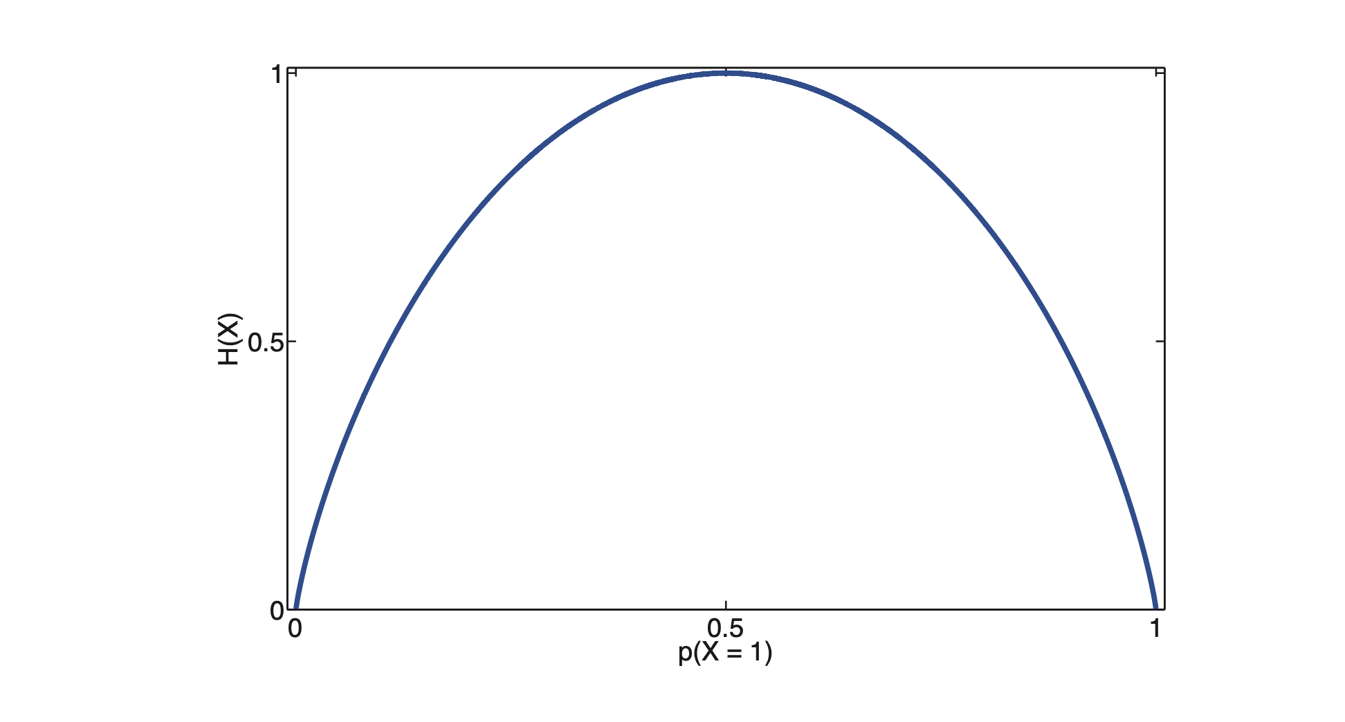
With the maximum value of \(1\) occurs when the distribution is uniform, with \(\theta = 0.5\), which happens in the fair coin. Therefore, we can say that the trial when tossing the coin reaches the highest certainty when using a fair coin. In the case that the coin is not fair, let us say with \(\theta = 0.7\), then:

\[\begin{aligned} \text{H}(X) &= -\big[0.7\log0.7 + 0.3\log0.3\big] \approx 0.8816 \end{aligned}\]

• Video Explanation

Cross-Entropy Estimation

• Information Theory:

  In the Information Theory aspect, the Cross-Entropy between two probability distributions \(p\) (true distribution) and \(q\) (estimated distribution) over the same underlying set of events measures the average number of bits needed to encode information from distribution \(p\) into of distribution \(q\). With two distributions \(p\) and \(q\), the Cross-Entropy is calculated by:

  \[\text{H}(p, \ q) = E_p[-\log q]\]

  For two probability distributions \(p = (p_1,\cdots, p_n)\) and \(q = (q_1,\cdots, q_n)\), we have the Cross-Entropy:

  \[\begin{align} \text{H}(p, q) = -\sum_{i=1}^np_i\log q_i \end{align}\]

  There are two important properties of Cross-Entropy:

  • \(\text{H}(p,\ q)\) reaches the minimum value when \(p = q\)
  • Cross-Entropy is highly sensitive to the difference. Specifically, the greater the difference between \(p_i\) and \(q_i\), the larger the value \(\text{H}(p,\ q)\) is and vice versa.

  Cross-Entropy is widely used to calculate the distance between two probability distributions. However, as it is a non-symmetrical function: \(\text{H}(p,\ q) \neq \text{H}(q, \ p)\), Cross-Entropy cannot be used as a distance metric.

• Probabilistic Machine Learning:

  In the machine learning aspect, as the objective is to build models so that the predicted \(\hat y\) is as close to the target \(y\) as possible (\(\hat y\) and \(y\) are both the probability distributions), Cross-Entropy is typically applied as the loss function to optimize the learning model.

  • For \(n\)-category classification task, where ground-truth label \(y\) is often encoded by the one-hot vector (meaning \(y=1\) at ground-truth class \(i\) and \(y=0\) otherwise). Over \(n\) classes, the Categorical Cross-Entropy Loss \(\mathcal{L}_{CE}\) is defined by:

    \[\mathcal{L}_{CE} = -\sum_{i=1}^ny\log(p_i)\]

    with \(p_i =\hat y\) is the Softmax probability that predicts the \(i^{th}\) class. However, with the one-hot encoding, \(y\) can be removed because we only want to keep \(p_i\) which comes with the right prediction. Therefore, over \(N\) data points, the Categorical Cross-Entropy Loss is defined by:

    \[\begin{equation} \mathcal{L}_{CE} = -\frac{1}{N}\sum_{i=1}^N\log(p_i) \end{equation}\]

  • For the binary classification task, where the ground-truth label \(y\) takes either the value of \(0\) or \(1\), the binary Cross-Entropy Loss \(\mathcal{L}_{BCE}\) is defined by:

    \[\begin{align} \mathcal{L}_{BCE} = -\frac{1}{N}\sum_{i=1}^N\big[y\log(p_i) + (1-y) \log(1-p_i)\big] \end{align}\]

    for \(N\) data points where \(p_i\) is the softmax probability for the \(i^{th}\) data point.

  • Video Explanation

Kullback–Leibler Divergence

The Kullback-Leibler Divergence (KL Divergence), also known as the relative entropy, is a typical statistical distance: a measurement of how distribution \(p\) is different from the distribution \(q\). Given two probability distributions \(p = (p_1,\cdots, p_n)\) and \(q = (q_1,\cdots, q_n)\), the KL divergence \(D_{KL}(p\mid \mid q)\) is defined by:

\[\begin{equation} \begin{aligned} D_{KL}(p\mid \mid q) &= \text{H}(p, \ q) - \text{H}(p) \\&= \sum_{i=1}^np_i\log q_i -\sum_{i=1}^np_i\log p_i = \sum_{i=1}^np_i\log \frac{p_i}{q_i} \end{aligned} \end{equation}\]

where \(\text{H}(p, \ q)\) is the cross-entropy between \(p\) and \(q\), and \(\text{H}(p)\) is the entropy of \(p\).

The KL Divergence is non-negative, and it is \(0\) if \(p\) and \(q\) are the same distribution, or equal “almost everywhere” in the case of continuous. Similar to the cross entropy, the KL Divergence is also non-symmetric \(D_{KL}(p\mid \mid q) \neq D_{KL}(q\mid \mid p)\) and thus cannot be used as a distance metric.

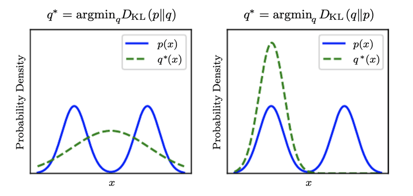
In Information Theory, especially in the sending message task, the cross entropy \(\text{H}(p,\ q)\) can be interpreted as the number of bits per message needed on average to encode events drawn from true distribution \(p\), if using an optimal code for distribution \(q\), while the KL Divergence \(D_{KL}(p\mid \mid q)\) measures the average number of extra bits per message, whereas \(\text{H}(p, \ q)\) measures the average number of total bits per message.

• The quantity of “bit” can be measured by Entropy by equation \((10)\)

Similar to the Cross-Entropy, KL Divergence can be applied in the Machine Learning aspect. Minimizing the KL Divergence is similar to minimizing the Cross Entropy. However, Cross-Entropy is more well-known and applied.

Intuition:

• How Cross-Entropy difference with the KL Divergence:

  What is the difference Cross-entropy and KL divergence?

• Video Explanation

Bonus: Wasserstein Distance

Since Cross-Entropy and KL-Divergence are non-symmetric, Wasserstein Distance is used to measure a distance between two probability distributions as a distance metric. It is also called the Earth Mover’s Distance (EM Distance), as it is informally interpreted as the minimum amount of work required to transform one distribution into one another.

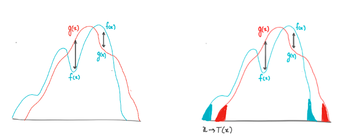
Wasserstein Distance is often used in Optimal Transport. The scope is beyond Information Theory. The detail of Wasserstein Distance is presented in this article:

Optimal Transport and Wasserstein Distance.pdf

---

References

• Blitzstein, Joseph K., and Jessica Hwang. Introduction to probability. Boca Raton, FL: Crc Press, 2015.
• Goodfellow, Ian, Yoshua Bengio, and Aaron Courville. Deep learning. MIT press, 2016.
• Murphy, Kevin P. Machine learning: a probabilistic perspective. MIT press, 2012.
• Ross, Sheldon. A first course in probability. Pearson, 2010.