Introduction to Probability - Part 1
- The basic principles of probability and counting
- Conditional Probability
- Bayes’s Theorem
- Random variables distribution
- Expectation and Variance
- Discrete Probability Distribution
- Continuous Probability Distribution
- Recap of basic probability
The basic principles of probability and counting
Basic counting
-
Permutation:
The permutation indicates how many different ordered arrangements can be made from a set of \(n\) items, calculated by:
\[\begin{equation} P(n) = n! \end{equation}\] -
Combination:
The combination indicates how many ways to select \(k\) items from a set of \(n\) items (\(k < n\)) without order arrangement, calculated by:
\[\begin{equation} \begin{aligned} \begin{pmatrix}n\\ k\end{pmatrix} = C(n,\ k) = \frac{n!}{k!(n-k)!} \end{aligned} \end{equation}\]-
For any positive \(n\) and \(k\) with \(k \leq n\), we also have:
\[\begin{aligned} \begin{pmatrix}n\\ k\end{pmatrix} = \begin{pmatrix}n\\ n - k\end{pmatrix} \end{aligned}\]and
\[\begin{aligned} k\begin{pmatrix}n\\ k\end{pmatrix} = n\begin{pmatrix}n-1\\ k-1\end{pmatrix} \end{aligned}\]
-
-
\(k\)-permutations of \(n\):
The \(k\)-permutation of \(n\) indicates many ways to select \(k\) items from a set of \(n\) items (\(k < n\)) with order arrangement, calculated by:
\[\begin{equation} \begin{aligned} P(n,\ k) = \frac{n!}{(n-k)!} \end{aligned} \end{equation}\] -
The binomial theorem:
\[\begin{equation} (x + y)^n = \sum_{k=0}^n \begin{pmatrix}n\\ k\end{pmatrix}x^ky^{n-k} \end{equation}\]
Basic probability
- Given two events \(A\) and \(B\), we have:
- \(A\cup B\) is the event that occurs if at least one of \(A\) or \(B\) occurs
- \(A\cap B\) is the event that occurs if both \(A\) and \(B\) occurs
- The complement \(A^c\) is the event that occurs if and only if \(A\) does not occur
-
De Morgan’s Law:
\[\begin{equation} \begin{aligned} (A\cup B)^c =A^c \cap B^c \\ \\ (A\cap B)^c =A^c \cup B^c \end{aligned} \end{equation}\]-
General form:
Given a set of events \(A_1, \ A_2, \cdots, \ A_n\), we have:
\[\begin{aligned} \left(\bigcup_{i=1}^n A_i\right)^c = \bigcap_{i=1}^n A_i \end{aligned}\] \[\begin{aligned} \left(\bigcap_{i=1}^n A_i\right)^c = \bigcup_{i=1}^n A_i \end{aligned}\]
-
-
Naive definition of probability:
\[P_\text{naive}(A) = \frac{|A|}{|S|} = \frac{\text{number of outcomes favorable to }A}{\text{total number of outcomes in }S}\] -
General definition of probability:
A probability space consists of a sample space \(S\) and a probability function \(P\) which takes an event. \(A \subseteq S\) (\(A\) is the subset of \(S\)) as input and returns \(P(A)\), a real number between \(0\) and \(1\), as output. The function \(P\) must satisfy the following axioms:
- \[P(\emptyset) = 0, \qquad P(S) = 1\]
-
If \(A_1, \ A_2, \cdots\) are disjoint events (mutually exclusive: \(A_i \cap A_j = \emptyset\) for \(i \neq j\)), then
\[P\left(\bigcup_{j=1}^\infty A_j\right) = \sum_{j=1}^\infty P(A_j)\]
Conditional Probability
-
With two events A and B, the probability of \(A\) given that the event \(B\) already happened is the “conditional probability of A given B” \(P(A\mid B)\), calculated by:
\[\begin{equation} P(A\mid B) = \frac{P(A\cap B)}{P(B)} \end{equation}\]- In general: \(P(A \mid B) ≠ P(B \mid A)\) when \(P(A) ≠ P(B)\)
-
Example:
- In August, the probability of a rainy day is \(0.8\). The probability there is a rainy day with clouds in the sky is \(0.6\). Thus, the probability that there is a rainy day when the sky cloud is:
Law of Addition and Multiplication
-
Multiplication rule: The joint probability of having both \(A\) and \(B\) occur is:
\[\begin{equation} P(A\cap B) = P(A, \ B) = P(A\mid B)\cdot P(B) \end{equation}\] -
Additional rule: The probability that two events \(A\) or \(B\) occur is:
\[\begin{equation} P(A\cup B) = P(A) + P(B) - P(A \cap B) \end{equation}\] -
Special cases:
- When the \(A\) and \(B\) are mutually exclusive (two events cannot happen at the same time):
- When \(A\) and \(B\) are not mutually exclusive and independent:
-
The cases with 3 events \(A\), \(B\), and \(C\):
\[\begin{aligned} P(A,B,C) &= P(A)\cdot P(B \mid A) \cdot P(C\mid A, B) \\ P(A \cup B \cup B) &= P(A) + P(B) + P(C) \\ & \quad - P(A \cap B) - P(A \cap C) - P(B \cap C) \\ & \quad + P(A \cap B \cap C) \end{aligned}\]
Independence of Events
- Independent events
-
\(A\) and \(B\) are two independent events if:
\[P(A \cap B) = P(A) \cdot P(B)\] -
If \(P(A) >0\) and \(P(B)> 0\), then:
\[P(A\mid B) = P(A)\] \[P(B\mid A) = P(B)\] -
If \(A\) and \(B\) are independent, then \(A\) and \(B^c\) are independent, \(A^c\) and \(B\) are independent, and \(A^c\) and \(B^c\) are independent.
-
- Conditional independent:
-
Assume that \(A\), \(B\), and \(C\) are three events. We say that events A and B are independent given event C if:
\[\begin{equation} P(A, B \mid C) = P(A \mid C) \cdot P(B \mid C) \end{equation}\]- This notion means that once we know event \(C\), the events \(A\) and \(B\) do not convey information about each other
-
“Independence” ≠ “Conditional independence”
-
“Event A and B are independent” does not mean that “A and B are independence given event C”
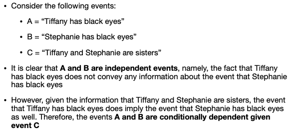
-
Events A and B can be dependent and yet they are independent given an event C
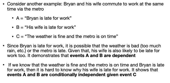
-
-
Bayes’s Theorem
-
With Bayes’s Theorem, \(P(A \mid B)\) can be calculated by:
\[\begin{equation} P(A\mid B) = \frac{P(B|A)\cdot P(A)}{P(B)} \end{equation}\]- Notations:
- \(P(A)\): the prior probability, namely, how probable the event \(A\) is before we have seen the data information \(B\)
- \(P(B \mid A)\): the likelihood, namely, conditional on event \(A\), how likely is that we would see data information \(B\)
- \(P(B)\): the marginal (unconditional) probability of \(B\) (regardless of whether event \(A\) holds or not)
- \(P(A\mid B)\): the posterior probability, namely, how probable the event \(A\) after we have seen the information \(B\)
- Notations:
- Variants of Bayes’s Theorem:
-
Odd form:
\[\frac{P(A \mid B)}{P(A^c \mid B)} = \frac{P(B \mid A)}{P(B \mid A^c)} \cdot \frac{P(A)}{P(A^c)}\]where \(A^c\) is the event that \(A\) does not hold
-
With 3 events \(A, \ B, \ C\), we have:
\[\begin{aligned} P(A \mid B, C) &= \frac{P(B \mid A, C) \cdot P(A \mid C)}{P(B \mid C)} \\&= \frac{P(A,B,C)}{P(B \mid C)} = \frac{P(B, C\mid A) \cdot P(A)}{P(B, C)} \end{aligned}\]
-
-
Understand better Bayes’s theorem:
- Examples:
-
In September, the probability of a rainy day is \(0.6\). The probability there is a cloudy day is \(0.3\). The probability that there are clouds on a rainy day is \(0.4\). Therefore, the probability that there is a rainy day when the sky cloud is:
\[P(rain \mid cloud) = \frac{P(rain) \cdot P(cloud \mid rain)}{P(cloud)} = \frac{0.6 \times 0.4}{0.3} = 0.8\] -
A particular test when someone has been using cannabis is \(90\%\) sensitive, leading to the true positive rate being \(0.9\), the test is also \(80\%\) specific, meaning the true negative rate is \(0.8\). Therefore, the test correctly identifies \(80\%\) of non-user as non-user. Assuming for a group of people, there are \(5\%\) that use cannabis, which is \(0.5\) prevalence. The possibility that random people test correctly as a cannabis user is:
\[P(User \mid Positive) = \frac{P(Positive\mid User)\cdot P(User)}{P(Positive)} = \frac{0.9 \times 0.05}{0.08} = 0.19\]
-
Law of Total Probability
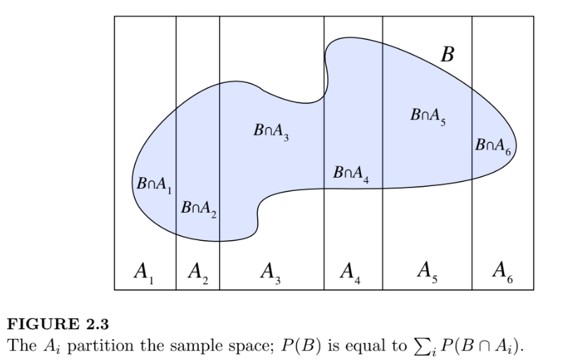
- \(\Omega\) denotes the set of all possible outcomes
-
Given an event space:
\[\Omega = B_1 \cup B_2 \cup B_3 \cup \cdots \cup B_m\]with an arbitrary event \(B \in \Omega\), we have the Law of Total Probability:
\[\begin{equation} \begin{aligned} P(B) &= \sum_{i=1}^mP(B\cap A_i) \\ &= \sum_{i=1}^mP(B\mid A_i) \cdot P(A_i) \end{aligned} \end{equation}\] -
Simpson’s Paradox
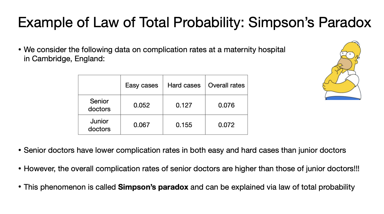
- Senior doctors take 213 easy cases, 102 hard cases, a total of 315 cases. While the junior doctors take 3375 cases including 3169 easy cases and 206 hard cases. Explain the paradox:
-
With \(A\) = {complication rates of senior doctors}
\[\begin{aligned} P(A) &= P(A \mid easy) \cdot P(easy) + P(A \mid hard) \cdot P(hard) \\ &= 0.052 \times \frac{213}{315} + 0.127 \times \frac{102}{315} = 0.076 \end{aligned}\] -
With \(B\) = {complication rates of junior doctors}
\[\begin{aligned} P(B) &= P(B \mid easy) \cdot P(easy) + P(B \mid hard) \cdot P(hard) \\ &= 0.067 \times \frac{3169}{3375} + 0.155 \times \frac{206}{3375} = 0.072 \end{aligned}\] -
Thus, we observe that the reason for Simpson’s paradox is:
- The junior doctors mostly perform easy cases with low complication rates
- The senior doctors have a higher fraction of hard cases, which leads to a higher overall rate
-
- Therefore, it is possible to have
- Senior doctors take 213 easy cases, 102 hard cases, a total of 315 cases. While the junior doctors take 3375 cases including 3169 easy cases and 206 hard cases. Explain the paradox:
-
In the standard case with two events \(A\), \(B\), with the Law of Total Probability, \(P(B)\) can be calculated by:
\[\begin{equation} P(B) = P(B \mid A) \cdot P(A) + P(B|A^c) \cdot P(A^c) \end{equation}\]- Example:
- \(50\%\) of emails are spam. A certain software can detect \(99\%\) of spam emails, with the probability that non-spam email is detected as spam email is \(5\%\). If an email is detected as spam email, what is the probability that this is in fact a non-spam email?
- Initially, we have:
- By the law of total probability:
-
With Bayes’s Theorem:
\[P(A \mid B) = \frac{0.05 \times 0.5}{0.52} \approx 0.048 = 4.8\%\]
- Example:
Bayesian Inference
-
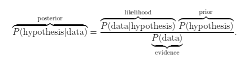
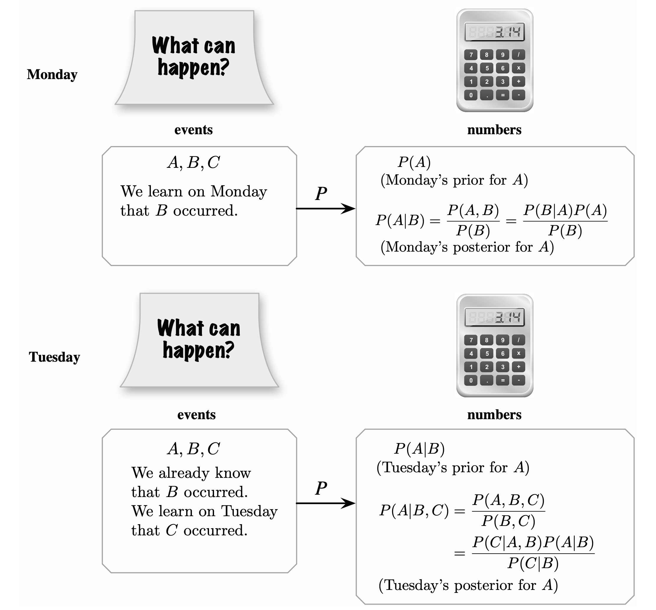
Bayesian inference is a method of statistical inference in which Bayes’s Theorem is used to update the probability of a hypothesis as more data become available:
Or:
\[Posterior = Likelihood × Prior ÷ Evidence\]
Random variables distribution
Given an experiment with sample space \(\Omega\), a random variable(s) (r.v.) is a measurable function \(X:S → E\) from a set of possible outcomes \(S \in \Omega\) to the real number \(E \in \mathbb{R}\)
Discrete Random Variable
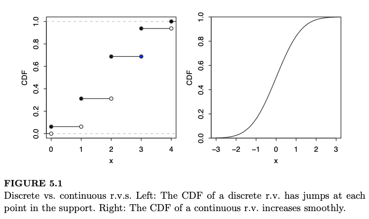
- A random variable that can take on at most a countable number of possible values (either finite or countably infinity) is said to be a discrete random variable.
-
For a discrete random variable \(X\), the probability mass function (p.m.f.) of \(X\) is the function \(p(a)\) gives the probability that a \(X\) takes on the value \(a\):
\[\begin{equation} p(a) = P(X = a) \end{equation}\]- If \(X\) is a discrete r.s., then the finite or countably infinity set of value \(x\) such that \(P(X = x) > 0\) is called the support of x
-
The cumulative distribution function (c.d.f.) of a random variables \(X\) (or more simply, the distribution function of \(X\)) is the function \(F_X(a)\) given by:
\[\begin{equation} F_X(a) = P(X \le a)= \underset{X \le a}{\sum}\ p(X) \qquad \qquad -\infty < x < \infty \end{equation}\]- We can write \(F_X(a)\) by \(F(a)\) for convenience if there is no risk of ambiguity
- c.d.f. is defined for all random variables, regardless it is discrete or continuous
- Examples:
-
Example 1: Suppose that we have an experiment of tossing the coin 3 times. Then we have
\(\Omega = \{HHH, \ HHT, \ HTH, \ HTT, \ THH, \ THT,\ TTH, \ TTT \}\).
If we let \(X\) denote the number of heads that appear, then \(X\) is a discrete random variable that takes one of the values \(E =\{0,..,3\}\).
- Thus, we have the p.m.f. of \(X\) with the respective probability:
- Given \(a = 2\), the c.d.f. of \(F(a)\) with the respective probability is given by:
-
Example 2: The p.m.f. of a random variable \(X\) is given by \(p(i) = c \frac{\lambda^i}{i!}, \ i = 0, 1, 2,\cdots,\) where \(\lambda\) is some positive value. Find (a) \(P(X=0)\) and \(F(3)\):
-
Since \(\sum_{i=0}^\infty p(i) = 1\), we have:
\[c\sum_{i=0}^\infty\frac{\lambda^i}{i!} = 1\]however, because \(e^x = \sum_{i=0}^\infty\frac{\lambda^i}{i!}\), then we have:
\[ce^\lambda = 1 \quad \Rightarrow \quad c = e^{-\lambda}\] -
Hence: \(P(X = 0) = e^{-\lambda}\frac{\lambda^0}{0!} = e^{-\lambda}\)
\[\begin{aligned} F(3) &= \sum_{X \leq 3}P(X) = P(0) + P(1) + P(2) + P(3)\\ &= e^{-\lambda} + \lambda e^{-\lambda} + \frac{\lambda^2 e^{-\lambda}}{2} + \frac{\lambda^3 e^{-\lambda}}{6} \\ &= \frac{\lambda^3 + 3 \lambda^2 + 6 \lambda + 6}{6}e^{-\lambda} \end{aligned}\]
-
-
Continuous Random Variable
- A random variable that has an uncountable number of possible values is said to be a continuous random variable. A random variable is continuous if its c.d.f. is differentiable (can be derivative at every point in its domain). Also, it must have a differentiable distribution.
-
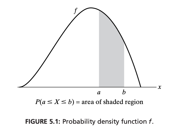
For a continuous r.v. \(X\) with c.d.f. \(F\), the probability density function (p.d.f.) \(f(x)\) of \(X\) is the derivative of \(F\), given by \(f(x) = F’(x)\). Thus, the p.d.f. \(f(x)\) can be defined for all real \(x \in (- \infty, \ \infty)\), having the property that, for any set \(B\) of real numbers:
\[\begin{equation} P(X \in B) = \int_B f(x)\ dx \end{equation}\]- The p.d.f. \(f\) of a continuous random variable must satisfy the following two criteria:
- Nonnegative: \(f(x) \ge 0\)
- Integrates to \(1\): \(\int_{-\infty}^{\infty} f(x) \ dx = 1\)
- The support of X, and of its distribution, is the set of all \(x\) where \(f(x) > 0\).
- The p.d.f. \(f\) of a continuous random variable must satisfy the following two criteria:
-
Special cases:
\[\begin{aligned} &P\left(X = a\right) = \int_{a}^{a} f(x) \ dx = 0 \\ &P\left(a \le X \le b\right) = \int_{a}^{b} f(x) \ dx \end{aligned}\] -
p.d.f. to c.d.f.: The c.d.f. \(F(a)\) of continuous r.v. \(X\) given the p.d.f. \(f(x)\) is calculated by:
\[\begin{equation} F(a) = P(X \le a) = \int_{-\infty}^a f(x)\ dx \end{equation}\] -
Examples:
-
Example 1: The amount of time in hours that a computer functions before breaking down is a continuous random variable \(X\) with the probability density function given by:
\[\begin{aligned} f(x) = \begin{cases} C(4x - 2 x^2) & 0 < x < 2 \\ 0 &\text{otherwise} \end{cases} \end{aligned}\]What is the value of \(C\) and calculate \(P(X > 1)\)?
Solution:
-
Since \(f(x)\) is a p.d.f., we must have:
\[\begin{aligned} \int_{-\infty}^{\infty} f(x) \ dx &= 1 \\ \Leftrightarrow \ C\int_{-0}^{2} (4x - 2x^2) \ dx &= 1 \\ \Leftrightarrow \ C\left[2x^2 - \frac{2x^3}{3}\right]\Bigg|_{x=0}^{x=2} &= 1 \\ \Rightarrow \ C &= \frac{3}{8} \end{aligned}\] -
Integrate the p.d.f. from \(1\) to \(+ \infty\), and we have:
\[\begin{aligned} P(X > 1) = \int_1^\infty f(x) \ dx = \frac{3}{8} \int_1^2(4x-2x^2) \ dx = \frac{1}{2} \end{aligned}\]
-
-
Example 2: A continuous random variable \(X\) follows the Logistic distribution with the following c.d.f.:
\[\begin{aligned} F(X) = \frac{e^x}{1 + e^x}, \qquad x \in \mathbb{R} \end{aligned}\]Find the p.d.f. \(f(x)\) and \(P(-2 < X < 2)\):
Solution:
-
To obtain the p.d.f., we differentiate the c.d.f., which gives:
\[\begin{aligned} f(x) = F(X)' = \frac{d}{dx} \left(\frac{e^x}{1 + e^x}\right) = \frac{e^x}{(1 + e^x)^2} \end{aligned}\] -
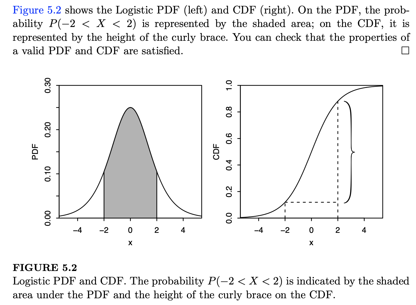
Integrate the p.d.f. from \(-2\) to \(2\), and we have:
\[\begin{aligned} P(-2 < X < 2) = \int_{-2}^2\frac{e^x}{(1+e^x)^2} \ dx = F(2) - F(-2) \approx 0.76 \end{aligned}\]
-
-
Independence of random variables
- If two random variables \(X\) and \(Y\) are independent, then knowing the value of \(X\) gives no information about the value of \(Y\), and vice versa.
-
Therefore, two random variables \(X\) and \(Y\) are independent for all \(x, y \in \mathbb{R}\) if:
\[\begin{equation} F_{X, Y}(x, y) = F_X(x)\cdot F_Y(y) \qquad \text{for all} \ x, y \end{equation}\]-
Equivalently, in the discrete case, given the p.m.f. \(P(X=x)\) and \(P(Y = y)\) and the joint probability mass function \(P(X = x, Y = y)\) exist:
\[P(X = x, Y = y) = P(X=x)\cdot P(Y=y)\] -
Or equivalently, in the continuous case, given the p.d.f. \(f_X(x)\) and \(f_Y(y)\) and the joint probability density functyion \(f_{X,Y}(x,y)\) exist:
\[f_{X, Y}(x, y) = f_X(x)\cdot f_Y(y)\]
-
-
Two random variables \(X\) and \(Y\) are conditionally independent given a random variable \(Z\) for all \(x, y \in \mathbb{R}\) and all \(z\) in the support of \(Z\) if:
\[\begin{equation} F_{X, Y \mid Z=z}(x, y) = F_{X \mid Z = z}(x) \cdot F_{Y\mid Z = z}(y) \qquad \text{for all } \ x, y, z \end{equation}\]-
Equivalently, in the discrete case, for any \(x, y \in \mathbb{R}\) and \(z \in \mathbb{R}\) with the p.m.f. \(P(Z=z) > 0\):
\[P(X = x, Y = y | Z = z) = P(X=x | Z=z)\cdot P(Y=y|Z=z)\] -
Or equivalently, in the continuous case, for all \(x, y \in \mathbb{R}\) and \(z \in \mathbb{R}\) with the p.d.f. \(f_Z(z) >0\):
\[f_{X, Y \mid Z}(x, y|z) = f_{X\mid Z}(x|z)\cdot f_{Y\mid Z}(y|z)\]
-
- Examples: A man and a woman decide to meet at a certain location. If each of them independently arrives at the time uniformly distributed between 12:00 and 13.00, find the probability that the first to arrive has to wait longer than 10 minutes.
-
Denote \(X\) and \(Y\) are, respectively, the time past 12:00 that the man and the women arrive. Thus, \(X\) and \(Y\) are two independent random variables, each of which is uniformly distributed over \((0, \ 60)\). We have the desired probability. \(P(X + 10 < Y) + P(Y + 10 < X) = 2P(X + 1 < Y)\) (by symmetry), calculated as follows:
\[\begin{aligned} 2P(X + 10 < Y) &= \underset{x + 10 < y}{\int\int}f(x,y)dx \ dy\\ &= 2\underset{x + 10 < y}{\int\int}f_X(x)f_Y(y)dx \ dy\\ &= 2\int_10^60\int_0^{y-10}\left(\frac{1}{60}\right)^2 dx \ dy \\ &= \frac{2}{360}\int_10^60(y-10)dy\\ &= \frac{25}{36} \end{aligned}\]
-
Expectation and Variance
Mean and median
- Given a list of number \(x_1, \ x_2, \cdots, x_n\), the arithmetic mean \(\bar{x}\) is defined by:
-
More generally, given the weight \(p_1, \ p_2, \cdots, p_n\) that add up to 1, the weighted mean (or mean as weighted sum) of \(x_1, \ x_2, \cdots, x_n\) is:
\[\begin{equation} \text{weighted-mean}(x) = \sum_{j=1}^np_j\cdot x_j \end{equation}\] -
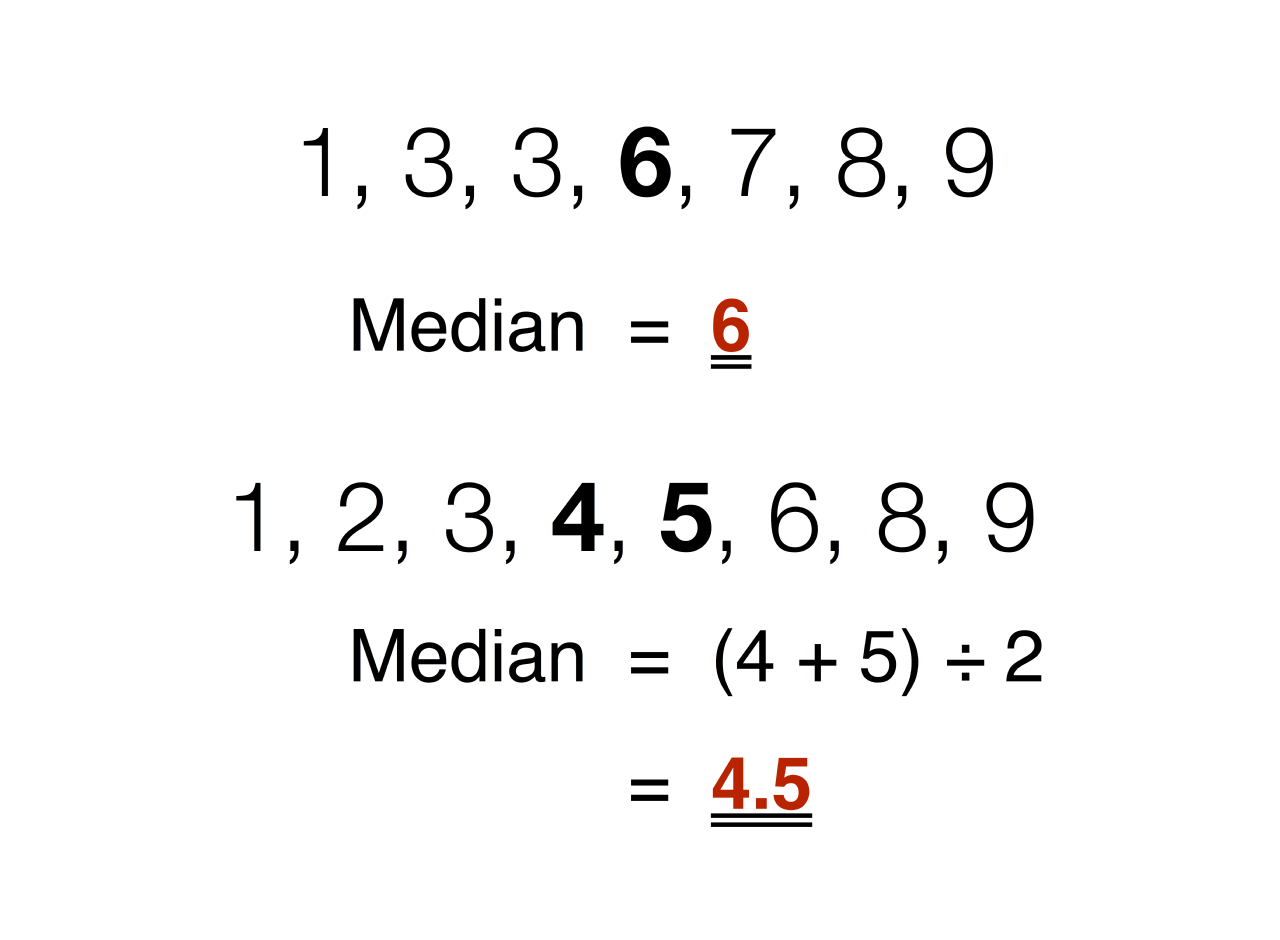
The median is the value that separates the first half and the second half of a sorted data sample, a population, or probabilistic distribution. It also may be considered “the middle” value. Given a list of sorted numbers \(x_1, \ x_2, \cdots, x_n\), there are two ways to find the median:
-
If \(n\) odd:
\[\text{median}(x) = x_{(n+1)/2}\] -
If \(n\) even:
\[\text{median}(x) = \frac{x_{(n/2)}+x_{(n+1)/2}}{2}\]
-
Expectation
The expectation (or expected value) indicates the center value of the distribution of a random variable.
-
Discrete random variable:
Given \(X\) is a discrete random variable having a p.m.f. \(p(x)\), then the expectation of \(X\), denoted as \(E[X]\) (or \(\mu\)), is defined by:
\[\begin{equation} \mu = E[X] = \sum_{x:p(x)>0}x\cdot p(x) \end{equation}\]Or it can also be written, if distinct possible values of \(X\) are \(x_1, \ x_2, \cdots, x_n\), by:
\[E(X) = \sum_{j = 1}^nx_j\cdot P(X=x_j)\]- Some theorems:
-
If two random variables \(X\) and \(Y\) share the same distribution, then:
\[E[X] = E[Y]\] -
For any random variables \(X, \ Y\) , and any constant \(c\), we have:
\[\begin{aligned} E[X + Y] &= E[X] + E[Y] \\ E[cX] &= c \cdot E[X] \end{aligned}\] -
Example: A school class of 120 students is driven in 3 buses to a symphonic performance. There are 36 students on one of the buses, 40 on another, and 44 on the third bus. When the buses arrive, one of the 120 is randomly chosen. Let \(X\) denote the number of students on the bus that are randomly chosen. Find the expectation of \(X\).
- Since the randomly chosen student is equally likely to be any of 120 students, it follows that: \(P(X = 36) = \frac{36}{120}; \quad P(X = 40) = \frac{40}{120}; \quad P(X = 44) = \frac{44}{120}\)
Thus, we have:
\[E[X] = 36\times\frac{3}{10} + 40\times\frac{1}{3} + 44\times\frac{11}{30} = \frac{1208}{30} = 40.2667\]
-
- Law of the unconscious statistician (LOTUS) for discrete r.v.:
- A function of a random variable is also a random variable. The Law of the unconscious statistician (LOTUS) is a theorem to calculate the expected value of a function \(g(X)\) of a random variable \(X\) given the probabilistic distribution of \(X\) but not \(g(X)\).
-
If \(X\) is a discrete random variable that takes on one of the values \(x_i, \ i \geq 1\), with respective probabilities \(p(x_i)\), then, for any real-valued function \(g\) from \(\mathbb{R}\) to \(\mathbb{R}\):
\[\begin{equation} E[g(X)] = \sum_i g(x_i)P(X = x_i) = \sum_i g(x_i)p(x_i) \end{equation}\] - Example: Let \(X\) denote a random variable that takes on any of the values \(-1, \ 0, \ \text{and} \ 1\) with respective probability: \(P(X = -1) = 0.2; \ P(X=0) = 0.5; \ P(X= 1) = 0.3\). Compute \(E[X^2 + 3]\)
-
We have:
\[\begin{aligned} E[X^2 + 3] &= [(-1)^2 + 3] \times 0.2 + (0^2 + 3) \times 0.5 + (1^2 + 3) \times 0.3 \\ &= 4 \times (0.2 + 0.3) + 3 \times 0.5 = 3.5 \end{aligned}\]
-
- Some theorems:
-
Continuous Random Variable:
Given \(X\) is a continuous random variable having the p.d.f. \(f(x)\), then, the expected value of \(X\) is:
\[\begin{equation} \mu = E[X] = \int_{-\infty}^{+\infty}xf(x) \ dx \end{equation}\]which is the balancing point of the p.d.f..
-
LOTUS for continuous r.v.:
If \(X\) is a continuous random variable and \(g\) is a function from \(\mathbb{R}\) to \(\mathbb{R}\), then:
\[\begin{equation} E[g(X)] = \int_{-\infty}^{+\infty}g(x)f(x) \ dx \end{equation}\]
-
Variance
- Variance summary is the distribution of a random variable, just like expectation. While the expectation shows the center of mass of a distribution, the variance shows how spread out that distribution is. The variance is denoted as \(\text{Var}(X)\).
-
Given the expectation value \(\mu = E[X]\) of a random variable \(X\), the variance is calculated by:
\[\begin{equation} \begin{aligned} \text{Var}(X) &= E[(X - \mu)^2]\\ &= E[X^2] - E[X]^2 \end{aligned} \end{equation}\] -
A useful identity is that for any constant \(a\) and \(b\):
\[\text{Var}(aX + b) = a^2\text{Var}(X)\] -
Also, variance is not linear, which means:
\[\text{Var}(X + Y) \neq \text{Var}(X) + \text{Var}(Y)\] -
The square root of the \(\text{Var}(X)\) is called the standard deviation, denoted as \(\text{SD}(X)\) or \(\sigma\), of \(X\):
\[\sigma = \text{SD}(X) = \sqrt{\text{Var}(X)} = \sqrt{E[(X - \mu)^2]}\] -
Discrete random variable:
Based on formula \((21)\) of the expected value \(\mu\) of a discrete random variable \(X\), the variance is calculated by:
\[\begin{equation} \sigma^2 = \text{Var}(X) = \sum_{i=1}^np(x_i)\cdot(x_i - \mu)^2 \end{equation}\] -
Continuous random variable:
Based on formula \((23)\), with the expected value \(\mu\) of a continuous random variable \(X\), we have:
\[\begin{equation} \sigma^2 = \text{Var}(X) = \int_{i=1}^n(x_i - \mu)^2f(x) \ dx \end{equation}\]-
Example: Find \(\mu\) and \(\sigma^2\) of a random variable \(X\), given the p.d.f.:
\[\begin{aligned} f(x) = \begin{cases} 2x \quad &\text{if} \quad 0 \leq x \leq 1\\ 0 &\text{otherwise} \end{cases} \end{aligned}\]We have:
-
Expectation:
\[\begin{aligned} \mu = E[X]= \int_0^1xf(x) \ dx = \int_0^1 2x^2 \ dx = \frac{2}{3} \end{aligned}\] -
Variance:
\[\begin{aligned} E[X^2] &= \int_0^1x^2f(x) \ dx = \int_0^1 2x^3 \ dx = \frac{1}{2}\\ \\ \sigma^2 &= \text{Var}(X) = \frac{1}{2} - \left(\frac{2}{3}\right)^2 = \frac{1}{18} \end{aligned}\]
-
-
Discrete Probability Distribution
A probability distribution is a statistical model that describes all the probabilities of all possible events that a random variable can take within range. Some distributions are so ubiquitous in probability and statistics that they have their own name.
-
A random variable \(X\) that is said to have the distribution \(A\) with parameter \(p\) is usually denoted as
\[X \sim A(p)\]which the symbol \(\sim\) is read as “is distributed as”
- Usually, a probability distribution function can be defined by two main parameters: expectation \(\mu\), and variance \(\sigma^2\). But there are cases with different sets of parameters.
- If \(X\) follows a certain probability distribution, said Uniform distribution, we can say \(X\) is a Uniform random variable
Discrete Uniform Distribution
- Discrete Uniform distribution* is closely connected to the naive definition of probability, described by picking a random number from a finite set of possibilities, where a finite number of values are equally likely to be observed, every one of \(n\) values has equal probability \(\frac{1}{n}\).
-
Let \(C\) be a finite, nonempty set of numbers, all values in \(C\) are equally likely. Choose one of these numbers uniformly at random. The random variable of getting a number \(X\) follows the Discrete Uniform distribution with parameter \(C\), denoted by \(X \sim \text{DUnif}(C)\). The p.m.f. of the distribution is:
\[\begin{equation} P(X=x) = \frac{1}{|C|} \end{equation}\] - The examples of the Discrete Uniform Distribution can be rolling a die, tossing a coin (this is a special case of Discrete Uniform Distribution called Bernoulli), or drawing a card from a desk
Bernoulli and Binomial Distribution
-
Bernoulli distribution:
A discrete random variable \(X\) is said to have the Bernoulli distribution with parameter \(p\) if \(X\) has only two outcomes \(X = 0\) and \(X = 1\), following the probability mass function of X given by:
\[\begin{equation} \begin{cases} p(1) = P(X=1) = p \\ p(0) = P(X=0) = 1 - p \end{cases} \end{equation}\]where \(0 \leq p \leq 1\) is the probability that the trial success. Therefore, \(X \sim \text{Bern}(p)\)
- The indicator random variable of an event \(A\) is the random variable which equals \(1\) if \(A\) occurs and \(0\) otherwise. The indicator r.v. of \(A\) is denoted by \(I_A \sim \text{Bern}(p)\) with \(p = P(A)\)
- An experiment where the outcome can be classified as either success or failure is often called a Bernoulli trial. Therefore, \(p\) is often called the success probability.
- The most famous example of Bernoulli distribution is the experiment when tossing a single coin. In that case: \(p=0.5\)
-
Binomial distribution:
Suppose that there are \(n\) independent Bernoulli trials performed with the same success probability \(p\). If discrete random variable \(X\) represents the number of successes that occur in the \(n\) trials, then \(X\) follows the Binomial distribution with parameters \(n\) and \(p\), denoted by \(X \sim \text{Bin}(n, \ p)\), where \(n\) is a positive number with \(0 \leq p \leq 1\). Then, the p.m.f. of \(X\) is:
\[\begin{equation} p(i) = \begin{pmatrix}n\\ i\end{pmatrix}p^i(1-p)^{n-i} \qquad \text{where } i = 0, 1,\cdots,n \end{equation}\]-
By the binomial theorem, all the probabilities sum to \(1\); that is:
\[\begin{aligned} \sum_{i=0}^\infty p(i) = \sum_{i=0}^n\begin{pmatrix}n\\ i\end{pmatrix}p^i(1-p)^{n-i} = [p + (1 - p)]^n = 1 \end{aligned}\] - Example: A pack of screws produced by a certain company will be defective with a probability \(0.02\), independently for each screw. The company sells the screws in packages of 10 and offers a money-back guarantee that at most \(1\) of \(10\) screws are defective. What proportion of packages sold must the company replace?
-
If \(X\) is the number of defective screws in a package, then \(X \sim \text{Bin}(10, \ 0.02)\). Hence, the probability that a package will have to be replaced is:
\[1 -p(0) - p_1) = 1 - \begin{pmatrix}10\\ 0\end{pmatrix}(0.02)^0 (0.98)^10 - \begin{pmatrix}10\\ 1\end{pmatrix}(0.02)^1 (0.98)^9 \approx 0.016\]
-
-
Expectation and variance:
If \(X \sim \text{Bin}(n, \ p)\), then:
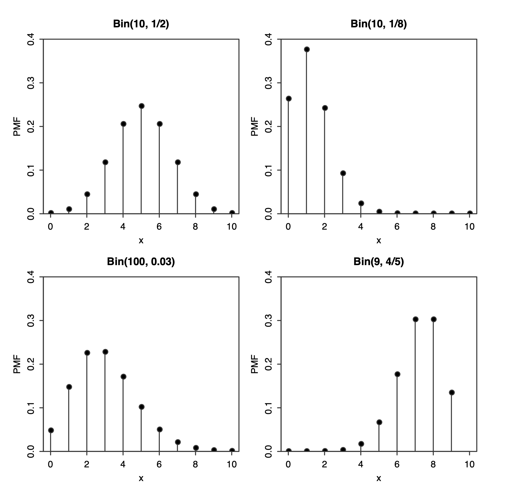
\[\begin{aligned} E[X] &= np\\ \text{Var}(x) &= np(1-p) \end{aligned}\] - Several Binomial p.m.f., given different sets of \((n, p)\):
-
Categorical and Multipomial Distribution
-
Categorical distribution:
Categorical distribution is the generalization of Bernoulli distribution. Thus, sometimes it can be referred as a generalized Bernoulli distribution or multinoulli distribution.
Given \(X\) is a discrete random variable that follows the Categorical distribution, \(X\) then takes on one of \(X\sim \text{Cat}_k(k,\ \boldsymbol{p})\) possible categories, with the probability of each category separately specified. Therefore: \(X\sim \text{Cat}_k(k,\ \boldsymbol{p})\) where \(\boldsymbol{p} = [p_1,\cdots, \ p_k]\).
- Note that all the probability \(p_1, \cdots, \ p_k\) must be in the range of \(0\) and \(1\), and all must sum \(1\).
-
The probability mass function of Categorical distribution is:
\[\begin{equation} p(i|\boldsymbol{p}) = \prod_{i=1}^kp_i^{[x = i]} \end{equation}\]where \([x = i]\) is in the Inverson bracket, indicates that:
\[[x=i] = \begin{cases} 1 \quad & \text{if } x=i \\ 0 & \text{otherwise} \end{cases}\] - A well-known example of the categorical distribution is the experiment that rolls a fair die, where each \(p(i) = \frac{1}{6}\)
-
Multinomial distribution:
It is the generalization of Binomial distribution, where multiple independent trials follow the Categorical distribution. Given \(X\) is a discrete random variable that follows the Multipomial distribution consisting of \(n\) Categorical trials that outcome \(k\) results independently, we denote \(X \sim \text{Mult}_k(n, \ \boldsymbol{p})\), with the p.m.f.:
\[\begin{equation} P(X_1=n_1,\ X_2=n_2,\cdots,\ X_k = n_k)= \frac{n!}{n_1!n2!\cdots n_k!}p_1^{n_1}p_2^{n_2}\cdots p_k^{n_k} \end{equation}\]whenever \(\begin{aligned}\sum_{i=1}^kn_i =n\end{aligned}\), with \(n_i\) is the number that result \(i\)-th happened.
-
Example: Suppose 9 fair dice are rolled. The probability that \(1\) appears three times, \(2\) and \(3\) appear twice each, \(4\) and \(5\) once each, and \(6\) not at all is:
\[\begin{aligned} \frac{9!}{3!2!2!1!1!0!}\left(\frac{1}{6}\right)^3\left(\frac{1}{6}\right)^2\left(\frac{1}{6}\right)^2\left(\frac{1}{6}\right)^1\left(\frac{1}{6}\right)^1\left(\frac{1}{6}\right)^0 = \frac{9!}{3!2!2!}\left(\frac{1}{6}\right)^9 = \frac{1}{419904} \end{aligned}\]
-
Hypergeometric Distribution
-
Suppose that a sample of size \(n\) is to be chosen randomly without replacement from an urn containing of \(m\) white balls and \(b\) black balls. If we let \(X\) denote the number of white balls selected, then \(X\) is said to have the Hergeometric distribution with parameters \((w, b, n)\), denoted by \(X \sim \text{HGeom}(m,\ b,\ n)\). The p.m.f. of \(X\) is:
\[\begin{equation} P(X = k) = \frac{\begin{pmatrix}m\\k\end{pmatrix}\begin{pmatrix}b\\n-k\end{pmatrix}}{\begin{pmatrix}w+b\\n\end{pmatrix}} \end{equation}\] -
Example: A purchaser of electrical components buys them in lots of size \(10\). It is his policy to inspect \(3\) components randomly from a lot and to accept the lot only if all \(3\) are non-defective. If \(30\%\) of the lots have \(4\) defective components and \(70\%\) have only 1, what proportion of lots does the purchaser reject?
-
Let \(A\) denote the event that the purchaser accepts a lot. Now we have:
\[\begin{aligned} P(A) &= P(A|\text{lot have 4 defectives})\frac{3}{10} + P(A|\text{lot have 1 defectives})\frac{7}{10}\\ &= \frac{\begin{pmatrix}4\\0\end{pmatrix}\begin{pmatrix}6\\3\end{pmatrix}}{\begin{pmatrix}10\\3\end{pmatrix}}\frac{3}{10} + \frac{\begin{pmatrix}1\\0\end{pmatrix}\begin{pmatrix}9\\3\end{pmatrix}}{\begin{pmatrix}10\\3\end{pmatrix}}\frac{7}{10} = \frac{54}{100} \end{aligned}\]
-
Poisson Distribution
-
A discrete random variable has the Poisson distribution with parameter \(\lambda > 0\), denoted by \(X \sim \text{Pois}(\lambda)\), if the p.m.f. of \(X\) is:
\[\begin{equation} p(k) = \frac{e^{-k}\lambda^k}{k!} \end{equation}\]-
We have the expectation and variance of the Poisson distribution are both equal to \(\lambda\):
\[\begin{aligned} \text{Expectation:} \qquad E[X] &= e^{-\lambda}\sum_{k=0}^\infty k\frac{\lambda^k}{k!} = e^{-\lambda}\sum_{k=1}^\infty k\frac{\lambda^k}{k!}\\ &= \lambda e^{-\lambda}\sum_{k=1}^\infty k\frac{\lambda^{k-1}}{(k-1)!} = \lambda e^{-\lambda}e^\lambda = \lambda \\ \text{Variance:} \qquad E[X^2] &= e^{-\lambda}\sum_{k=0}^\infty k^2\frac{\lambda^k}{k!} = e^{-\lambda}e^\lambda\lambda(1 +\lambda) = \lambda(1 + \lambda)\\ \Rightarrow \quad \text{Var}(x) &= E[X^2] - E[X]^2 = \lambda(1 + \lambda) - \lambda^2 = \lambda \end{aligned}\]
-
- The Poisson distribution is often used in situations when counting the number of successes in a particular region or interval of time, or there are a large number of trials, each with a small probability of success.
- For example:
- The number of emails you received in an hour. Imagine, there are \(3.6 \times 10^6\) seconds in an hour, but in any specific millisecond, it is unlikely that you will get an email.
- The number of chips in a chocolate chip cookie, if we divide the cookie into small cubes; where the number of cubes is large, but the probability of getting a chocolate chip inside a single cube is small.
- Then, the parameter \(\lambda\) is interpreted as the rate of occurrence of these rare events. In these examples, \(\lambda\) could be \(20\) emails per hour or \(10\) chips per cookie
- In general, the Poisson distribution may be used as an approximation for a Binomial distribution with parameters \((n, p)\) where \(n\) is large and \(p\) is small enough so that \(np\) is of moderate size, by letting \(\lambda = np\)
-
Specifically: if \(X \sim \text{Bin}(n, \ p)\) and we let \(n \rightarrow \infty\) and \(p \rightarrow 0\) such that \(\lambda = np\) remains fixed, then the p.m.f. of \(X\) converges to the \(\text{Pois}(\lambda)\) p.m.f.. Therefore:
\[P(X = k) \rightarrow \frac{e^{-\lambda}\lambda^k}{k!}\]
-
- For example:
- Examples:
- Example 1: Suppose that the number of typographical errors on a single page of this book has a Poisson distribution with parameter \(\lambda = \frac{1}{2}\). Calculate the probability that there is at least one error on this page:
-
Let \(X\) denote the number of errors on this page, we have:
\[\begin{aligned} P(X \geq 1) = 1 - P(X = 0) = 1 - e ^\frac{1}{2}\frac{\frac{1}{2}^0}{0!} \approx 0.393 \end{aligned}\]
-
- Example 2: At least how many people are required in order to have a 50-50 chance that two people would have birthdays within one day of each other?
- The probability that any two people have birthdays within one day of each other is \(\begin{aligned}\frac{3}{365}\end{aligned}\) (choose a birthday for the first person, then the second person needs to be born on that day, the day before, or the day after)
- There are \(\begin{pmatrix}m \\ 2 \end{pmatrix}\) possible pairs, so the number within-one-day matches is approximately \(\text{Pois}(\lambda)\) where \(\begin{pmatrix}m \\ 2 \end{pmatrix}\frac{3}{365}\).
-
Therefore, to have a 50-50 chance of having a within-one-day birthday, we have:
\[\begin{aligned} &P(X \geq 1) = 1 - P(X = 0) = 1 - e^{}\approx 0.5 \\ &\Rightarrow e^{-\begin{pmatrix}m \\ 2 \end{pmatrix}\frac{3}{365}} \approx 0.5 \Rightarrow m \approx 14 \end{aligned}\]
- Example 1: Suppose that the number of typographical errors on a single page of this book has a Poisson distribution with parameter \(\lambda = \frac{1}{2}\). Calculate the probability that there is at least one error on this page:
Continuous Probability Distribution
Continuous Uniform Distribution
-
Similar to the discrete case, a continuous random variable \(X\) follows the continuous Uniform Distribution on the interval \((a, b)\), denoted by \(X \sim \text{Unif}(a,b)\), is a completely random number between \(a\) and \(b\), if its p.d.f. is:
\[\begin{equation} f(x) = \begin{cases} \frac{1}{b-a} \qquad &\text{if } x \in [a,\ b]\\ 0 & \text{otherwise} \end{cases} \end{equation}\]-
The c.d.f. of the distribution í the accumulated area under the p.d.f., which is
\[F(x) = \begin{cases}0 &\text{if } x \leq a \\ \frac{x-a}{n-a} \qquad &\text{if } x \in [a, \ b] \\ 1 &\text{if } x \geq b \end{cases}\]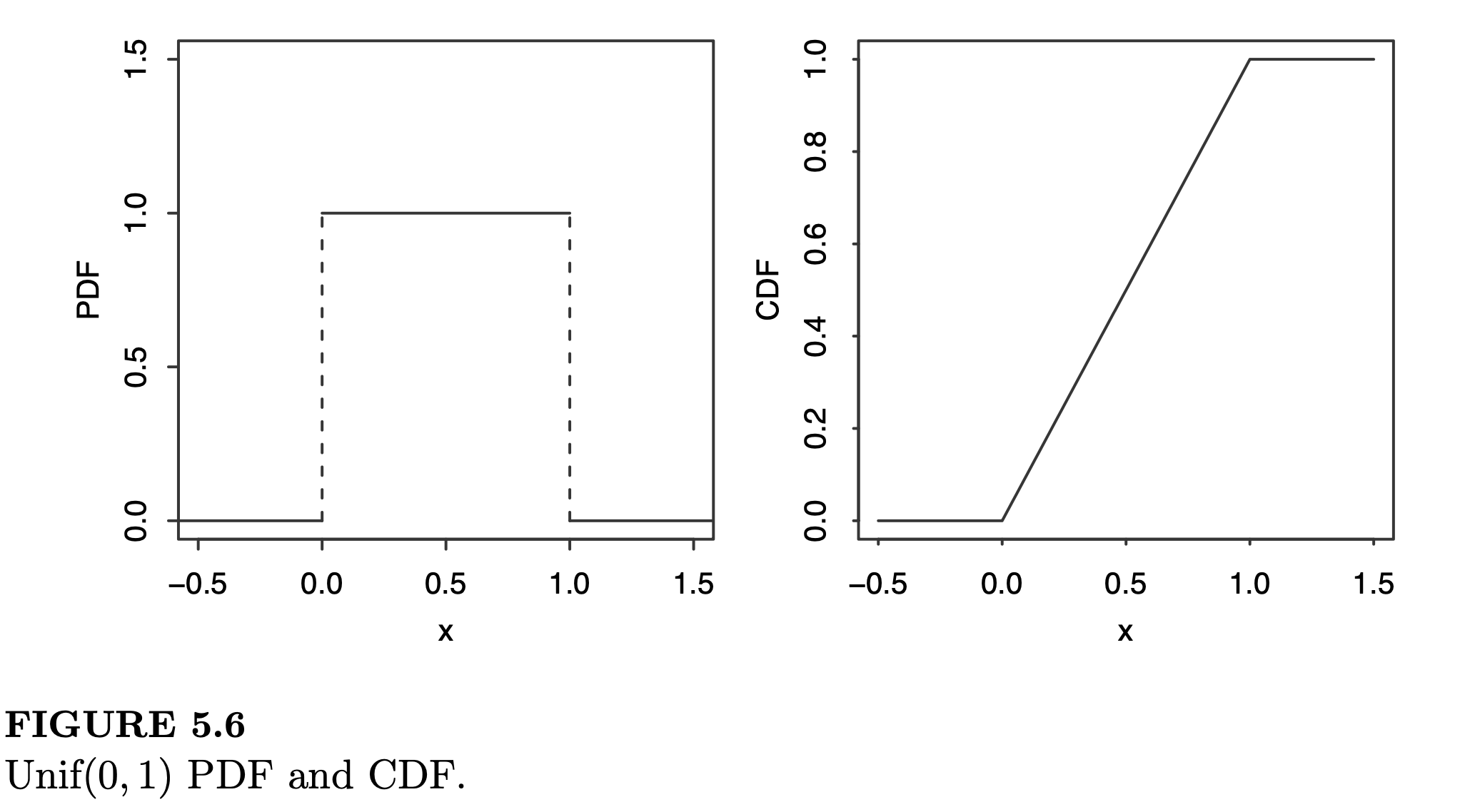
-
-
A good example of uniform distribution is an idealized random number generator. However, as every variable has an equal chance of happening, there is an infinity number of points that can exist, even in a small range.
Gaussian Distribution
- Gaussian Distribution (or Normal Distribution) is the most famous distribution and is extremely widely used in statistics
- The Central Limit Theorem says that, under very weak assumptions, the sum of a large number of independent and identically distributed random variables (discrete or continuous) has an approximately Normal distribution
- Moreover, in practice, many random phenomena obey, at least approximately, a normal distribution
- The Central Limit Theorem says that, under very weak assumptions, the sum of a large number of independent and identically distributed random variables (discrete or continuous) has an approximately Normal distribution
-
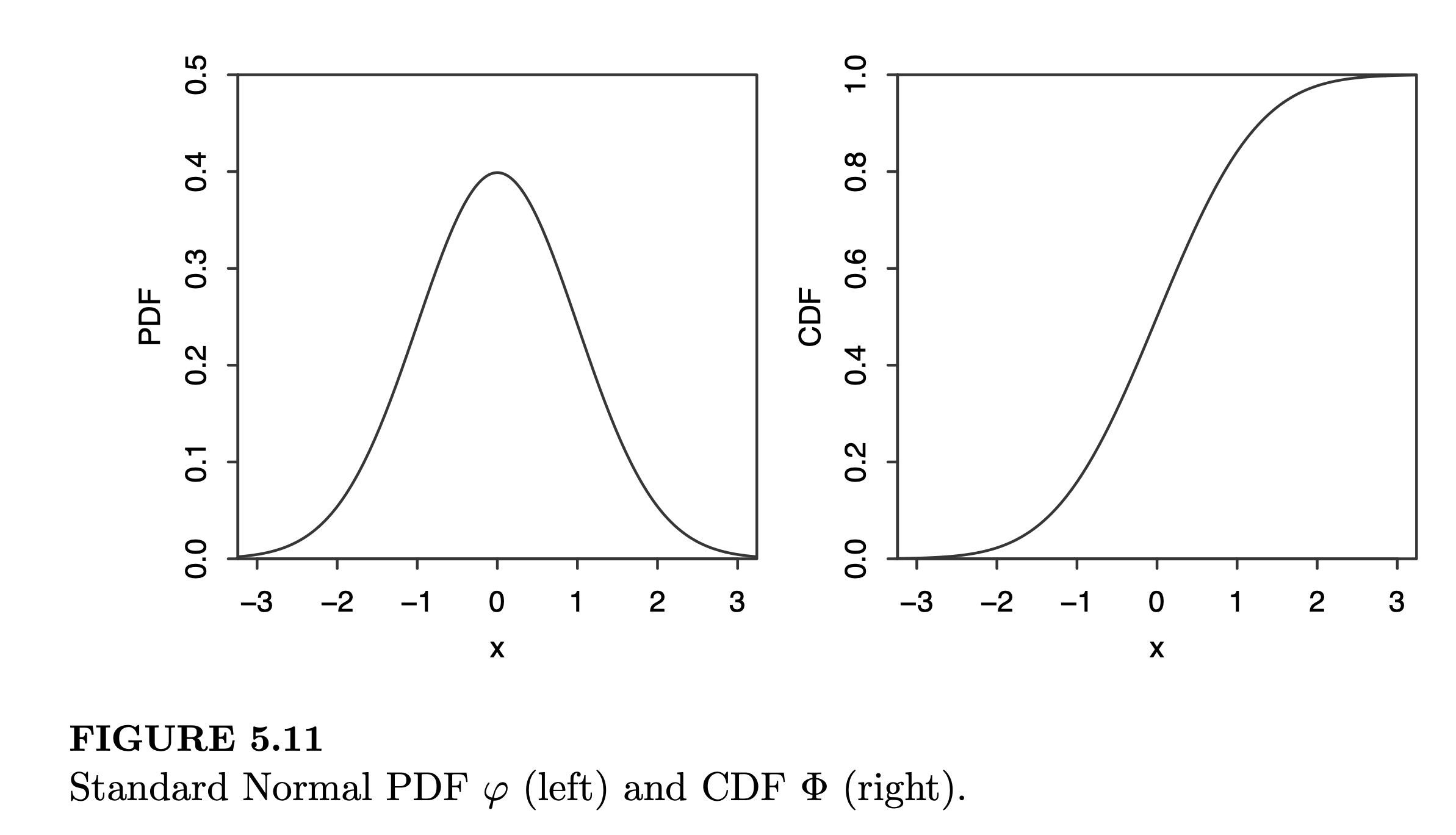
Standard Normal Distribution: A continuous random variable \(Z\) is said to have the standard Normal Distribution \(Z \sim \mathcal{N}(0,1)\) if its p.d.f. is given by:
\[\begin{align} \varphi(z) = \frac{1}{\sqrt{2\pi}}e^{-z^2/2} \end{align}\]-
The c.d.f. of a Normal Distribution, often denoted as \(\Phi\), is the accumulated area under the p.d.f., calculated by:
\[\begin{equation} \Phi(z) = \int_{-\infty}^z\varphi(t)\ dt = \int_{-\infty}^z\frac{1}{\sqrt{2\pi}}e^{-t^2/2} dt \end{equation}\]
-
Expectation and Variance:
\[\begin{aligned} E[X] &= \frac{1}{\sqrt{2\pi}}\int_{-\infty}^{+\infty}ze^{-z^2/2} \ dz \\ & = -\frac{1}{\sqrt{2\pi}}e^{-z^2/2}\big|_{-\infty}^{+\infty}\\ &= 0 \end{aligned}\] \[\begin{aligned} \text{Var}(Z) &= E[Z^2] - E[Z]^2\\ &= \frac{2}{\sqrt{2\pi}}\int_{0}^{+\infty}z^2e^{-z^2/2} \ dx \\ &= \frac{2}{\sqrt{2\pi}}\left(-ze^{-z^2/2}\bigg|_0^\infty + \int_0^\infty e^{-z^2/2} \ dz \right) \\ &= \frac{2}{\sqrt{2\pi}}\left(0 + \frac{\sqrt{2\pi}}{2}\right) = 1 \end{aligned}\]
-
-
Normal Distribution with variance and expectation: If \(Z \sim \mathcal{N}(0,1)\), a continuous random variable \(X = \mu + \sigma Z\) is said to follow the Normal Distribution with expectation \(\mu\) and variance \(\sigma^2\) , denoted by \(X \sim \mathcal{N}(\mu,\ \sigma^2)\). Thus, its p.d.f. is given by:
\[\begin{equation} f(x) = \varphi \left(\frac{x - \mu}{\sigma}\right)\frac{1}{\sigma}= \frac{1}{\sqrt{2\pi\sigma^2}}e^{-(x - \mu)^2/2\sigma^2} \end{equation}\]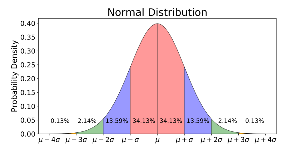
- The 68-95-99.7% rule: If \(X \sim \mathcal{N}(\mu, \ \sigma^2)\), then:
- The Normal approximation to the Binomial Distribution:
- When \(n\) large, a binomial random variable with parameters \(n\) and \(p\) will approximately follow the same distribution as a normal random variable with the same mean \(\mu = np\) and variance \(\sigma^2 = np(1-p)\) ** as the binomial (this is one case of the Central Limit Theorem)
-
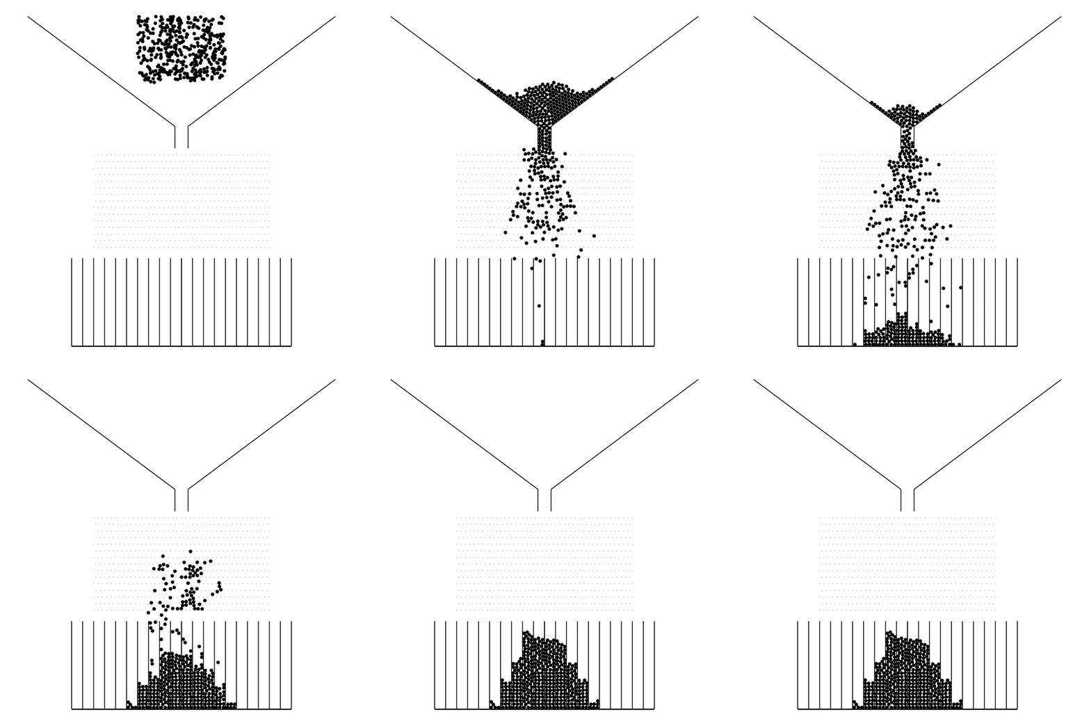
The DeMoivre-Laplace limit theorem: If \(S_N\) denotes the number of successes that occur when \(n\) independent trials perform, each resulting with probability \(p\), then, for any \(a < b\):
\[\begin{aligned} P\left(a \leq \frac{S_n - np}{\sqrt{}np(1-p)}\leq b \right) \rightarrow \Phi(b) - \Phi(a)\\ \end{aligned} \quad \text{as} \quad n \rightarrow \infty\]-
One example to visualize the theorem is the Galton Board, which can be observed by this GIF:
-
- Example: Let \(X\) be the number of times that a fair coin that is flipped 40 times lands on heads. Find the probability that \(X=20\) using the normal approximation and then compare it with the extract solution
-
Because the binomials is a discrete integer-valued random variable, whereas the normal is a continuous random variable, it is best to write \(P(X = i)\) as \(P(i - 1/2 < X < i + 1/2)\) before applying the normal approximation. Doing so gives:
\[\begin{aligned} P(X=20) &= P(19.5 \leq X \leq 20.5)\\ &= P\left(\frac{19.5 - 20}{\sqrt{10}}<\frac{X - 20}{\sqrt{10}}<\frac{20 - 20}{\sqrt{10}}\right)\\ &\approx P\left(-0.16<\frac{X - 20}{\sqrt{10}}<0.16\right)\\ &\approx \Theta(0.16) - \Theta(-0.16) \approx0.1272 \end{aligned}\]On the other hand, the extract result is:
\[\begin{aligned}P(X=20)=\begin{pmatrix}40\\20\end{pmatrix}\left(\frac{1}{2}\right)^{40}\approx 0.1254\end{aligned}\]
-
Exponential Distribution
- The Exponential Distribution often arises as the distribution of the amount of time until some specific event occurs. For instance, the amount of time (starting from now) until an earthquake occurs, or until a new war breaks out, ect.
-
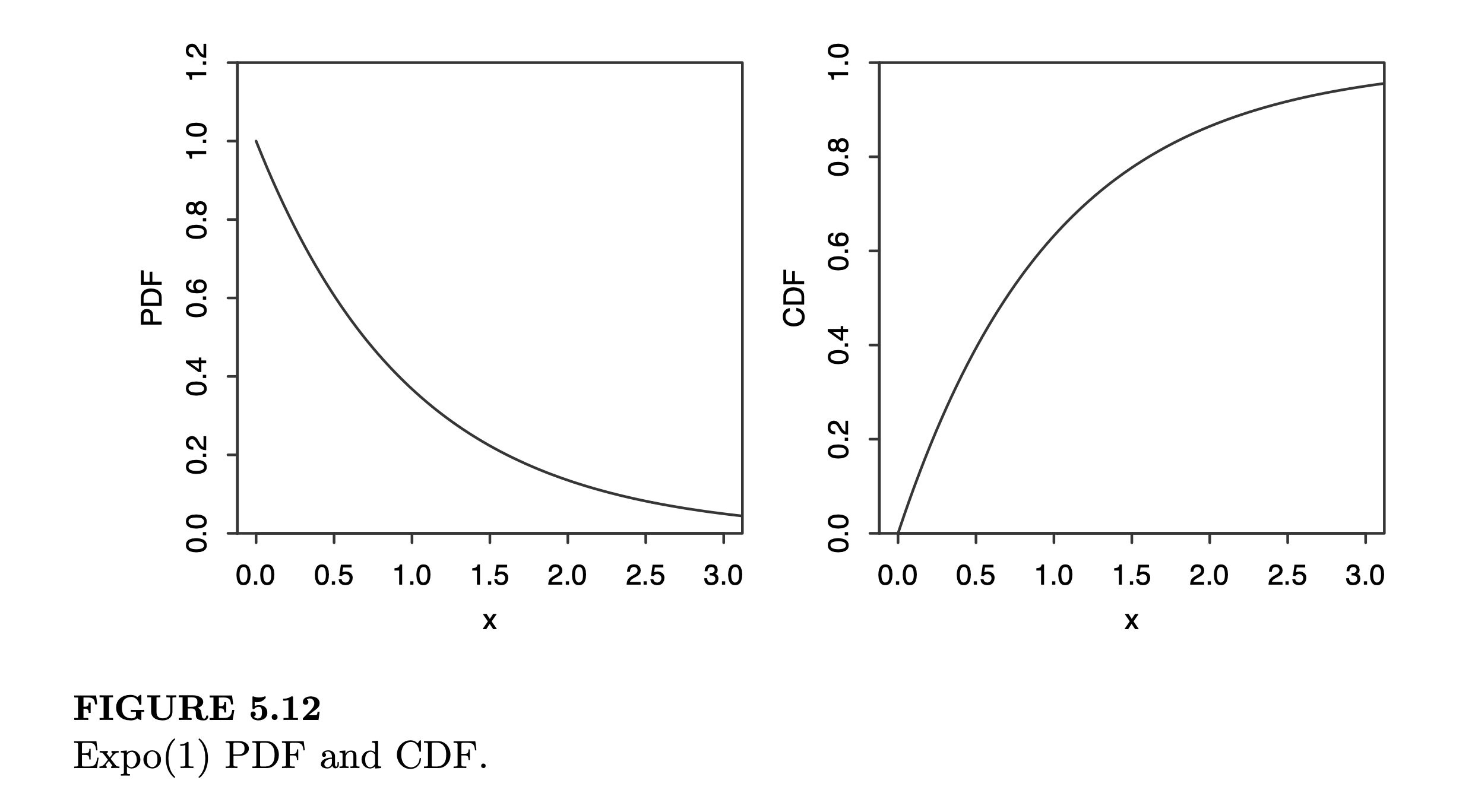
A continuous random variable X follows the Exponential Distribution \(X \sim \text{Expo}(\lambda)\) with parameter \(\lambda >0\) if its p.d.f. is:
\[\begin{equation} \begin{aligned} f(x) = \lambda e^{-\lambda x} \qquad x > 0 \end{aligned} \end{equation}\] -
The cossesponding c.d.f. is:
\[F(x)= 1 - e^{-\lambda x} \qquad x > 0\]
-
Expectation and variance:
\[\begin{aligned} E[X] = \frac{1}{\lambda};\quad\qquad \text{Var}(X) = \frac{1}{\lambda^2} \end{aligned}\] -
Example: Suppose that a length of a phone call in minutes is an exponential random variable with \(\lambda = \frac{1}{10}\). If someone arrives immediately ahead of you at a public telephone booth, find the probability that you have to wait: (a) more than 10 minutes; (b) between 10 and 20 minutes:
-
Let \(X\) denote the length of the call made by the person in the booth, we have:
\[P(X > 10) = 1 - F(10) = e^{-1} \approx 0.368\] \[P(10 < X<20) = F(20) - F(10) = e^{-1} - e^{-2} \approx 0.233\]
-
Gamma Distribution
-
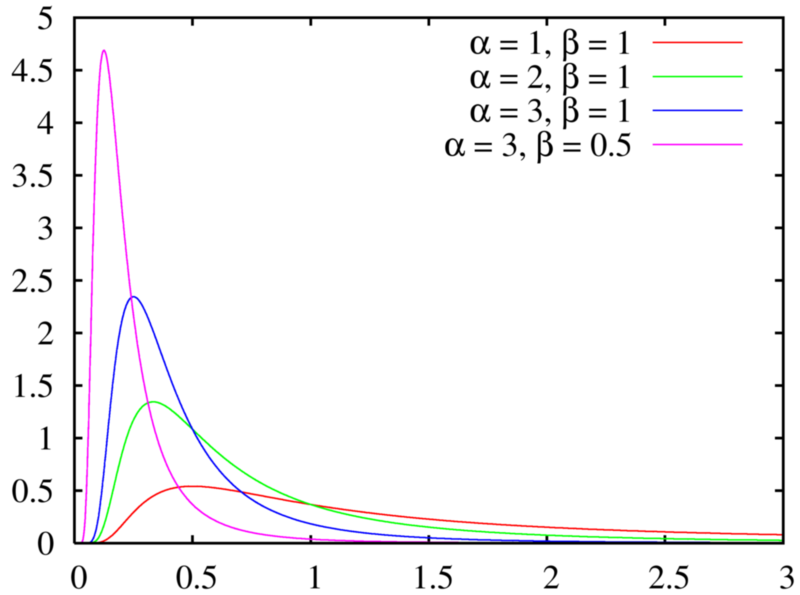
A random variable \(X\) is said to have Gamma distribution with parameter \(\alpha > 0; \ \beta > 0\), denoted as \(X \sim \Gamma(\alpha; \beta)\) if its p.d.f. is given by:
\[\begin{equation} f(x; \alpha, \beta) = \frac{\beta e^{-\beta x}(\beta x)^{\alpha - 1}}{\Gamma(\alpha)} \qquad x > 0 \end{equation}\]where \(\Gamma(\alpha)\), called the gamma function, is calculated by:
-
For integral values \(\alpha\) (discrete):
\[\Gamma(\alpha) = (\alpha - 1)!\] -
For real values \(\alpha\) (continuous):
\[\begin{aligned}\Gamma(\alpha) = \int_0^\infty t^{\alpha - 1}e^{-t} \ dt \end{aligned}\]
-
-
Expectation and variance:
\[\begin{aligned} E[X] = \frac{\alpha}{\beta};\quad\qquad \text{Var}(X) = \frac{\alpha}{\beta^2} \end{aligned}\]
Beta Distribution
-
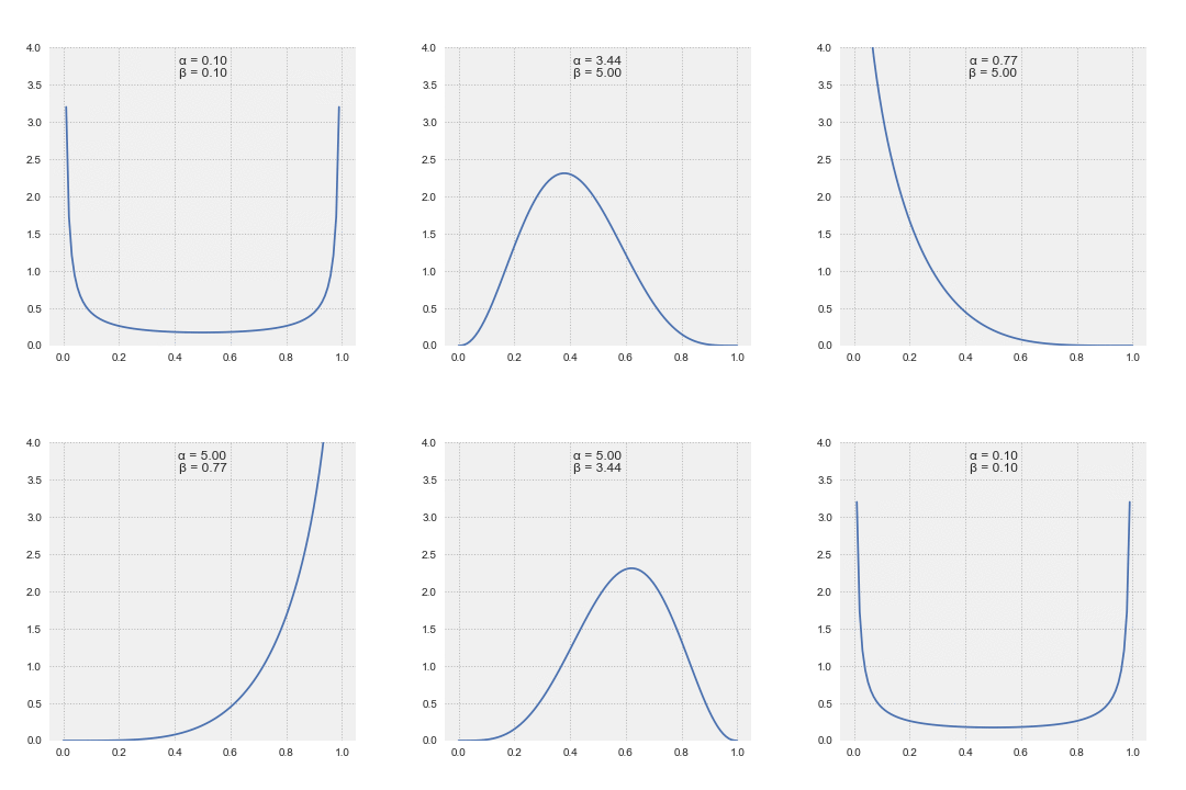
A random variable \(X\) is said to have Beta distribution with parameter \(\alpha > 0; \ \beta > 0\), denoted as \(X \sim \Beta(\alpha; \beta)\) if its p.d.f. is given by:
\[\begin{equation} f(x; \alpha, \beta) =\frac{1}{B(\alpha,\ \beta)}x^{\alpha - 1}(1-x)^{\beta - 1} \qquad 0 \leq x \leq 1 \end{equation}\]where \(\Beta(\alpha, \beta)\), called the beta function, is a normalization constant to ensure that the total probability is \(1\), calculated by:
\[\begin{aligned} B(\alpha, \beta) = \frac{\Gamma(\alpha)\Gamma(\beta)}{\Gamma(\alpha+\beta)} = \int_0^1x^{\alpha - 1}(1 - x)^{\beta - 1}\ dx \end{aligned}\] -
Expectation and variance:
\[\begin{aligned} E[X] = \frac{\alpha}{\alpha + \beta};\quad\qquad \text{Var}(X) = \frac{\alpha\beta}{(\alpha+\beta)^2(\alpha+\beta+1)} \end{aligned}\]
Recap of basic probability
Four fundamental concepts in probability
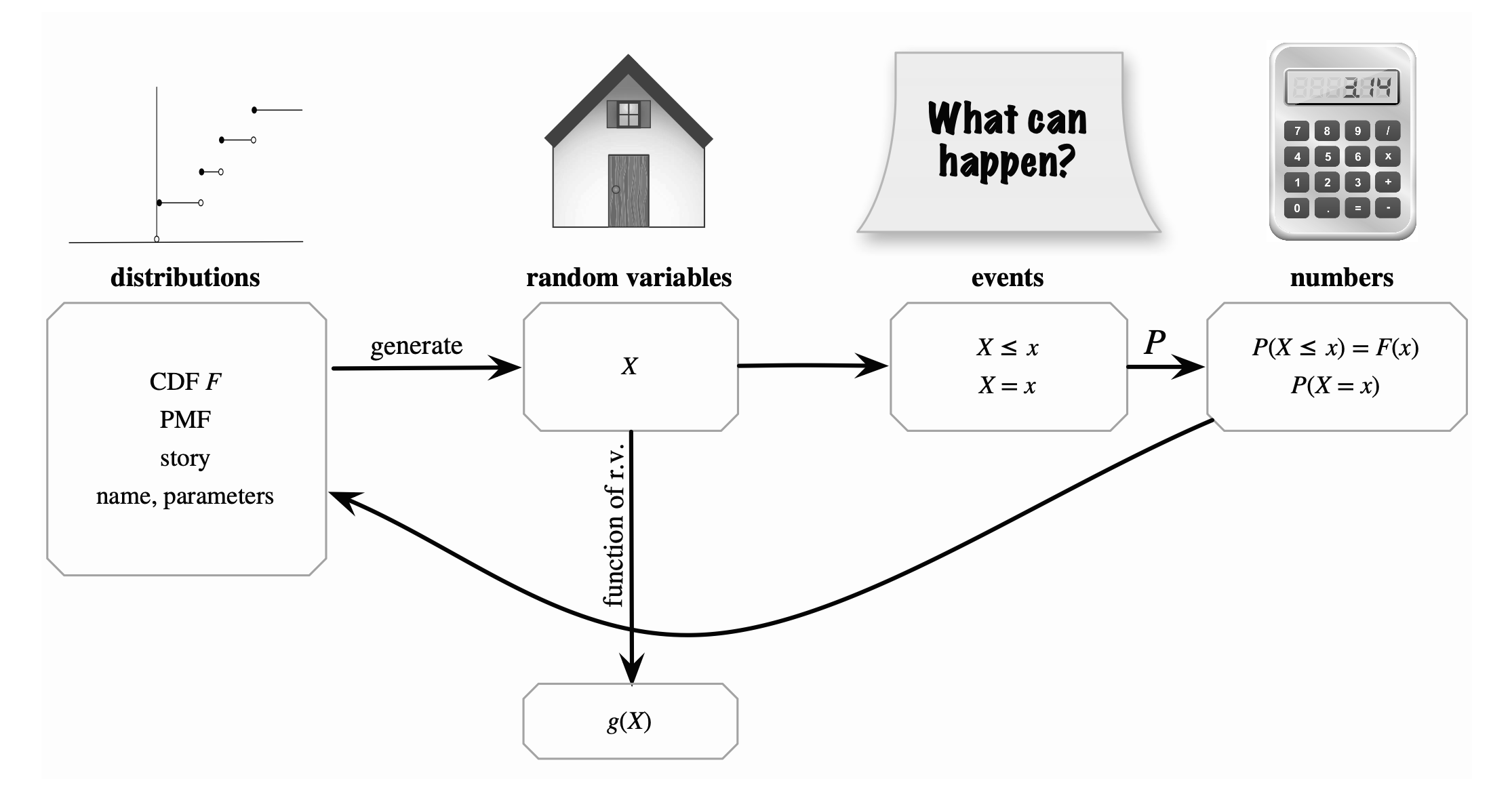
- The connections between four fundamental concepts in probability:
- From the distribution, we can obtain the distribution function c.d.f. \(F\)
- From the c.d.f., we can generate the random variables \(X\), or other random variables by taking the function of \(X\).
- There are various events \(x\) describing the behavior of \(X\). We mostly interest in the event \(X \leq x\) and \(X = x\).
- Then, we can calculate the value number of the probability of these events, by Bayesian rules for example.
- Knowing the probability of these events for all \(x\) gives us the c.d.f. and the p.m.f./p.d.f. of the random variable \(X\), thus describing the distribution of the random variable.
Bayesian reasoning
Random variable
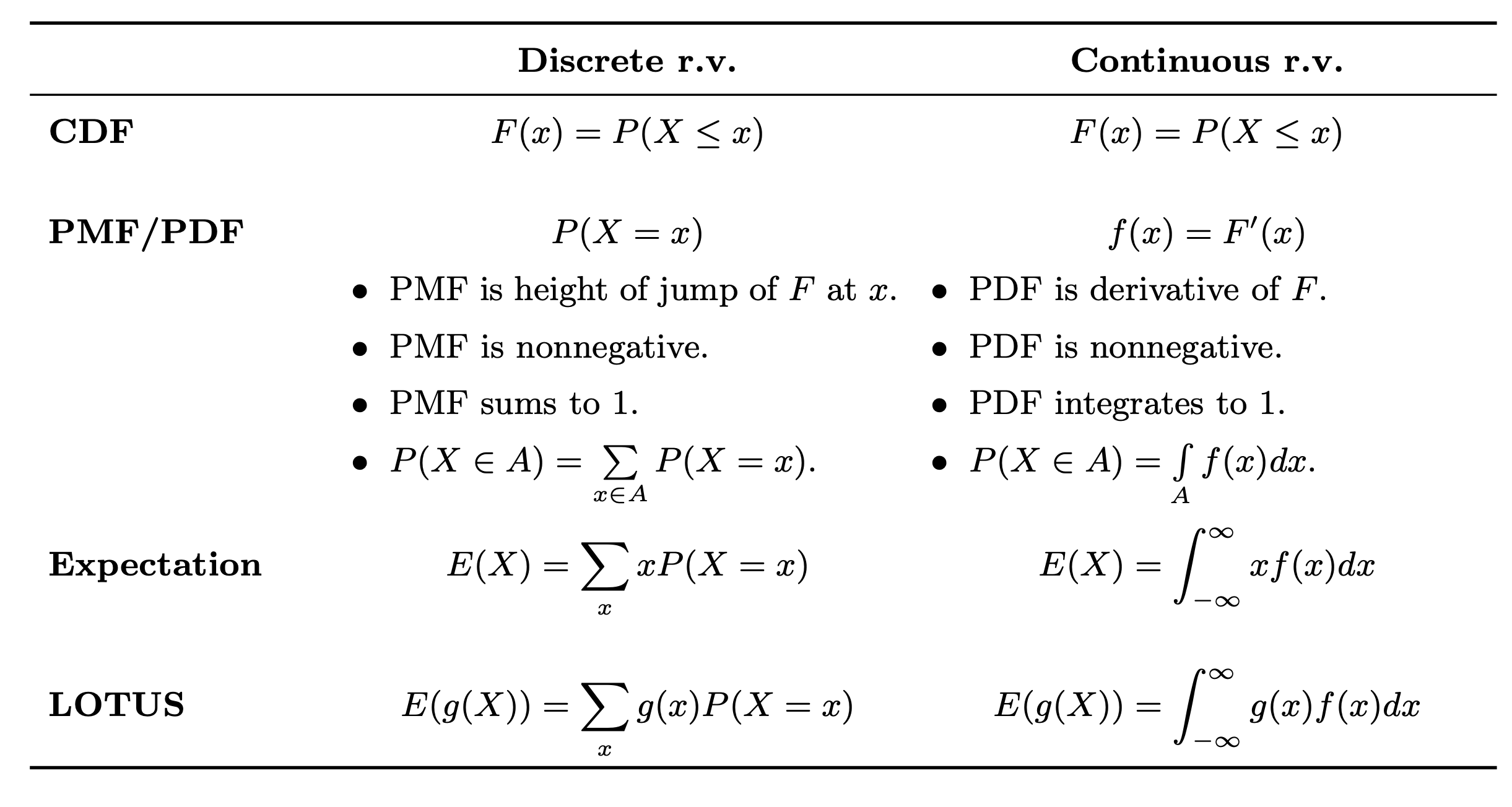
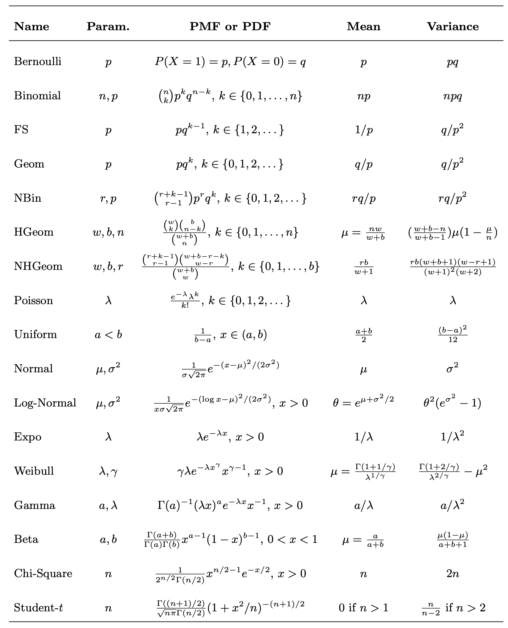
Table of Distributions
Enjoy Reading This Article?
Here are some more articles you might like to read next: