A list of important notations/symbols appear in this blog, arrange on the priority:
\(\phi(.)\): standard Gaussian probability density function (p.d.f.):
\[\phi(z) = \frac{1}{\sigma\sqrt{2\pi}}e^{-\frac{1}{2}\left(\frac{z - \mu}{\sigma}\right)^2}\]\(\Phi(.)\): standard Gaussian cumulative density function (c.d.f.):
\[\Phi(z) = \int_{-\infty}^z\phi(z')dz'\]Bayesian optimization routines rely on a statistical surrogate model of the objective function, whose beliefs guide the algorithm for the optimum result. Bayesian optimization has found an advantage in optimizing objects that:
One example application that raises the need for Bayesian Optimization is hyperparameter tuning problem. Consider crafting a complex machine learning model – say a deep neural network (DNN) – from training data. To ensure success, the model’s hyperparameter must be carefully tuned. One effective setting can only be identified via trial-and-error: by training several models with different configurations/settings and evaluating their performance on a validation dataset. But it cost time and resources.
The search for the best hyperparameter can be considered one of the procedures of mathematic optimization, with the DNN as an objective function. However, this optimization problem has many challenges, including:
Evaluation cost, in terms of time and resources
Multiple local optima, as the function is not convex and many combinations of hyperparameters come with locally optimal
Noise affection, as the deep neural network may return different values given the same set of hyperparameters, especially with the stochastic gradient descent.
No derivatives, as many hyperparameters are both discrete (number of layers, number of units per layer) or continuous (learning rate, weight decay), and there are no easy and inexpensive ways to propagate gradients between training/validation process
Conditional variable, as some hyperparameters are dependent on the settings of others
Bayesian optimization can deal with the problems that have these challenges. Furthermore, it can deliver impressive performance even when optimizing complex “black box” objectives given severely limited observation budgets. The core idea is to build a statistical model \(\mathcal{N}\) that is able to describe the uncertainty of the function \(f\) we are optimizing. By considering this model, we can find the next location to sample the function \(f\) by optimizing a much cheaper function. Based on the observation from the newly chosen location, we can update \(\mathcal{N}\) to reduce the uncertainty of \(f\), thus making it approximate with the objective function. This can be done with Bayesian inference. The process continues until we are sufficiently certain of where is the global optimal point of \(f\) through \(\mathcal{N}\).
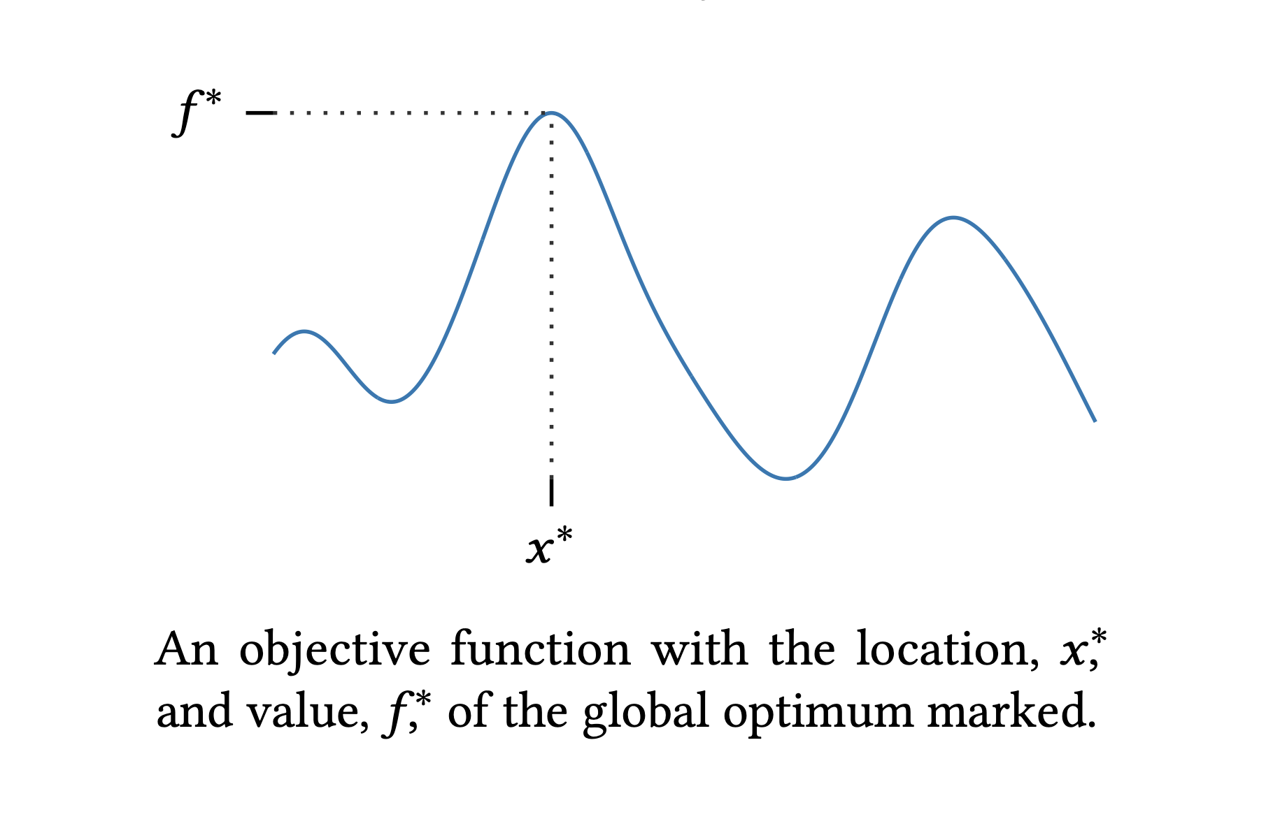
Given an unknown objective function \(f(x)\) defined on the domain of interest \(\mathcal{X}\). The goal of optimization is to search for the optimal value point \(x^* \in \mathcal{X}\) attaining with the global maximal \(f^*\):
\[\begin{equation} \begin{aligned} x^* &=\underset{x \in \mathcal{X}}{\arg \max}\ f(x) \\ f^* &= \underset{x \in \mathcal{X}}{\max}f(x) = f(x^*) \end{aligned} \end{equation}\]In global optimization, \(\mathcal{X}\) is often a compact subset of \(\mathbb{R}\), but in Bayesian optimization, \(\mathcal{X}\) can be an unusual search space that involves categorical or conditional inputs.
As \(f\) is unknown, instead of having a know functional form or even being computable directly, we can only access to a mechanism revealing some information about \(f\) at identified points on demand. That makes the optimization problem becomes black-box.
Fundamentally, mathematic optimization is a sequence of decisions: on each step, we must choose where to make our next decision and when to stop making decisions. Mathematic optimization often has a structure of sequential optimization, finding the optimal point based on a sequence of optimization experiments. The main algorithm of sequential optimization is described as follows, which are 3 main steps within a loop:
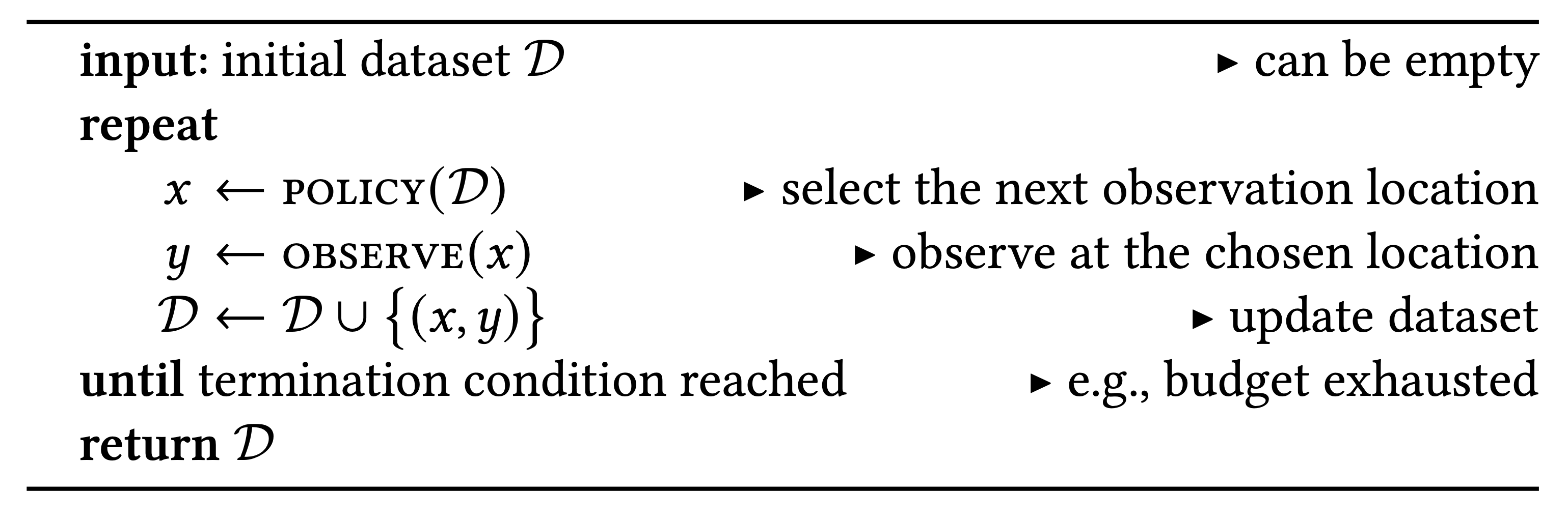
Optimization policy: examines any already gathered data \(\mathcal{D} = \{(x, y)_{1,\cdots,n}\}\) and select the next location \(x_{n+1}\)
Observation model: conduct observation (alternative function) at point \(x\) to guide the search for optimal point \(x^*\) of \(f\). As \(f\) cannot be observed directly and noises (imperfect stimulation, statistical approximation,\(\cdots\)) prevent the observation from yielding the exact value, we made an assumption that the observation model follows a stochastic mechanism depending on \(f\).
Termination: deciding whether to continue with another step (iteration) or terminate immediately, which is made at the end of the step
The central idea of Bayesian optimization is to build a model that can be updated and queried to drive optimization decisions, based on Bayesian inference, which is an inductive process whereby we can continue to refine our belief through additional observation.
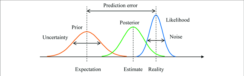
Given an unknown function \(f\). Let \(\mathcal{D} = (x, y)\) denote the available data. Since \(f\) is unobserved, we treat it as a latent random variable with a prior \(p(f)\), which captures a priori beliefs about probable values for \(w\) before any data is observed. Given data \(\mathcal{D}\) and a likelihood \(p(\mathcal{D}\mid f)\), we can then infer a posterior \(p(f \mid \mathcal{D})\) using Bayes’ rule:
\[\begin{equation} p(f \mid \mathcal{D}) = \frac{p( \mathcal{D} \mid f)\cdot p(f) }{p(\mathcal{D})} \end{equation}\]This posterior represents our updated beliefs about \(f\) after observing the data \(\mathcal{D}\). The marginal likelihood \(p(\mathcal{D})\), or the evidence, does not depend on \(f\) and is therefore simply a normalizing constant.
Bayesian Optimization is a sequential optimization framework to search for the optimal point \(x^*\) of a black-box function \(f\), including two key ingredients:
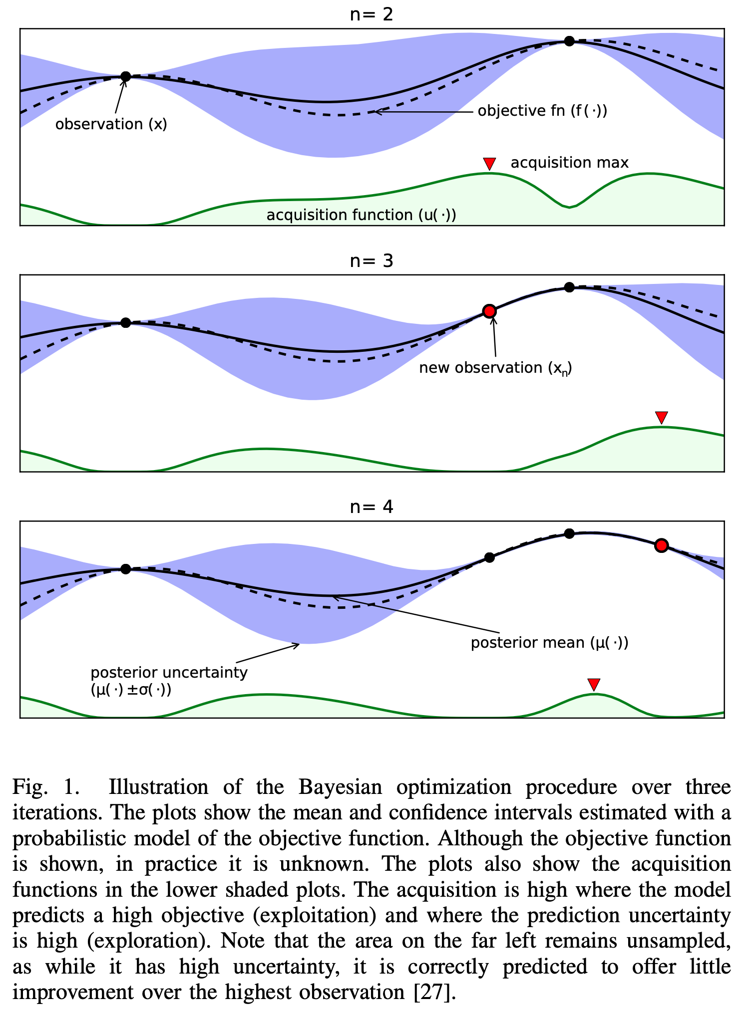
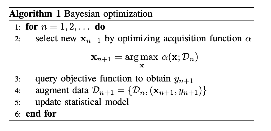
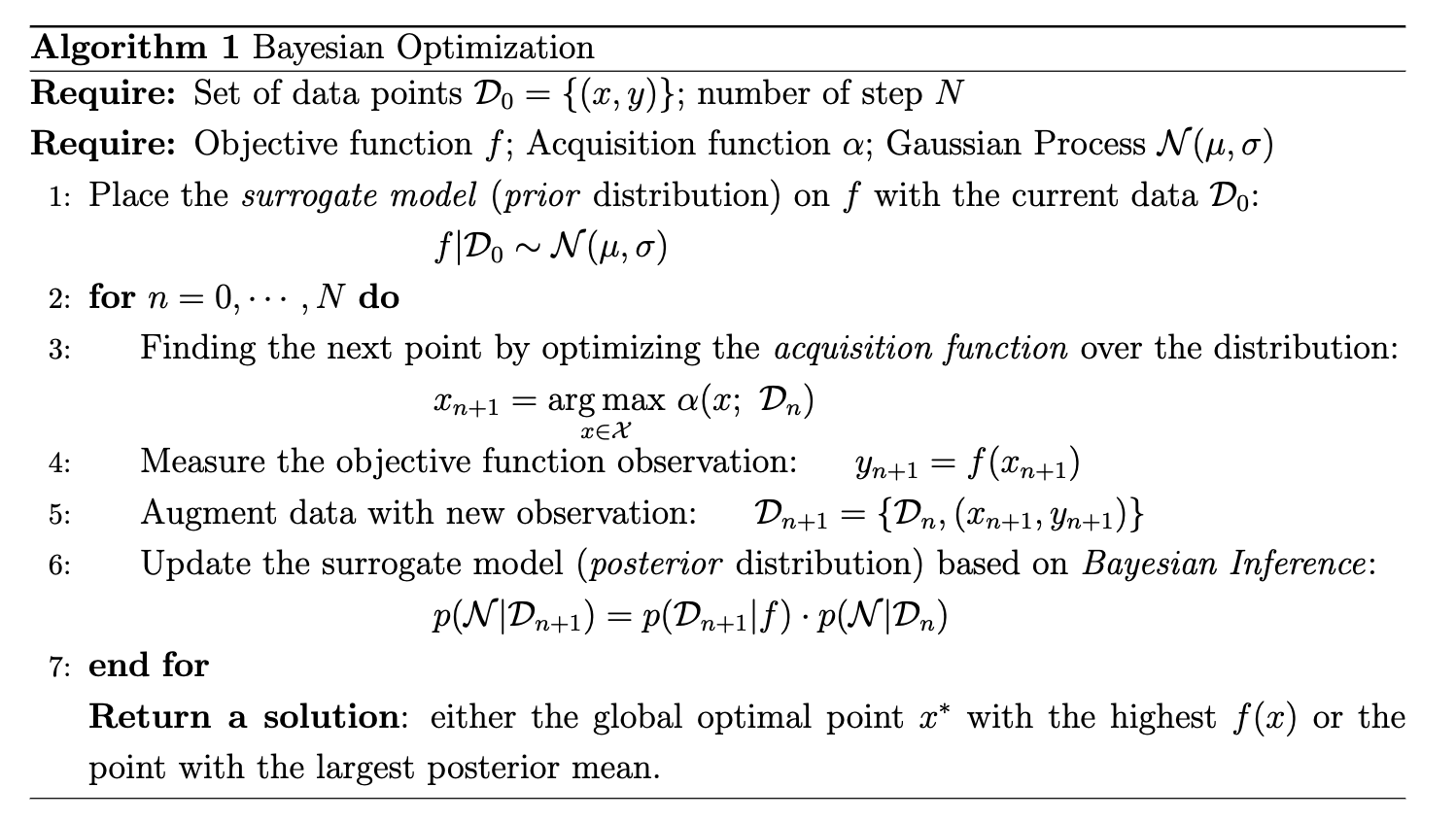
In short, the goal of Bayesian optimization is to build a probabilistic model over an unknown function that is able to update itself to drive the optimization decision by producing more data, with the new data can be either (i) selected on a certain area that probably has a high value here (exploitation) and (ii) selected on the uncertain area that might have a higher value there (exploration). Below is a simple algorithm of Bayesian Optimization:
As the objective function \(f\) cannot be optimized directly, one surrogate model is required for the replacement. This surrogate model allows us to (i) flexibly describe the objective function that needs to be optimized, (ii) estimate the uncertainty about the function, and (iii) can be updated to become approximate with the objective function for optimization. Based on observed data, we can compute a posterior distribution over the function \(f\) for such criteria. Among various methods, Gaussian Processes Regression stays the most famous choice for the surrogate model.
A very nice graphic of how surrograte model (Gaussian Process) updates.
In the following section, we discuss the mechanisms of the Gaussian Process, including how to place priors distribution over the objective function with prior observations and update their priors in light of the new observation.
Gaussian Process Regression is a Bayesian statistical approach for modeling functions. The Gaussian process \(\text{GP}(\mu,\ K)\) is a non-parametric model that is fully characterized by its prior mean function \(\mu: \mathcal{X} \rightarrow \mathbb{R}\) and its positive semi-definite covariance matrix (or kernel) \(K: \mathcal{X} \times \mathcal{X} \rightarrow \mathbb{R}\). The mean function determines the expected function value \(y = f(x)\) at any location \(x\), serving as a location parameter representing the function’s center tendency. The covariance function determines how deviations from the mean are structured, encoding expected properties of the function’s behavior.
The mean and covariance functions of the process allow us to compute any finite-dimensional marginal distribution on demand. With a finite set of data point \(\mathbf{x} = \{x_i\}_{i=1}^n\) and the corresponding observed values \(\mathbf{y} = f(\mathbf{x})\), Gaussian Process assumes that the distribution on \(\mathbf{y}\) follows the multivariate Gaussian with parameters determined by the mean and covariance functions, resulting in:
\[\begin{equation} \begin{aligned} \mathbf{y} \mid \mathbf{x} \sim \mathcal{N}\big(\mu, \ K\big) \end{aligned} \end{equation}\]The distribution on \(\mathbf{y}\) can be considered as a prior distribution on observed data \(\mathbf{x}\), with the elements of the mean vector \(\mu\) and the covariance matrix \(K\) are defined by \(\mu(x)= \mathbb{E}[f(x)]\) and \(K_{i,j}:=k(x_i, x_j) = \mathbb{E}\left[\big(f(x_i) - \mu(x_i)\big).\big(f(x_j) - \mu(x_j)\big)\right]\). This makes \(K\) the Gram matrix associate with \(\mathbf{x}\). The full expression of \((3)\) is:
\[\begin{aligned} \begin{bmatrix} y_1 \\ \vdots \\ y_n \end{bmatrix} \sim \mathcal{N}\left(\begin{bmatrix} \mu(x_1) \\ \vdots \\ \mu(x_n) \end{bmatrix}, \begin{bmatrix} k(x_1, x_1) &\cdots &k(x_1, x_n)\\ \vdots &\ddots &\vdots \\ k(x_n, x_1) &\cdots &k(x_n, x_n) \end{bmatrix} \right) \end{aligned}\]Suppose we already have \(n\) data points \(\mathbf{x} = \{x\}_{i=1}^n\), observed by \(\mathbf{y} = f(\mathbf{x})\) without noise, result in a prior distribution on \(\mathbf{y}\). Consider we have a new, arbitrary data point \(x\), observed by \(y = f(x)\) and we wish to infer the posterior distribution on \(y\). By the properties for Gaussian Process, \(\mathbf{y}\) and \(y\) are a jointly Gaussian:
\[\begin{bmatrix}y \\ \mathbf{y} \end{bmatrix} \sim \mathcal{N}\left(\begin{bmatrix} \mu(x) \\ \mu(\mathbf{x}) \end{bmatrix}, \begin{bmatrix} K(x, x) \quad K(x, \mathbf{x})\\ K(\mathbf{x}, x)\quad K(\mathbf{x}, \mathbf{x}) \end{bmatrix} \right)\]Based on Bayesian theorem \((2)\), we can find the expression of the posterior distribution by:
\[\begin{align} y \mid x, \mathbf{x} &\sim \mathcal{N}\big(\mu_n(x), \sigma_n^2(x)\big)\\ \end{align}\]where
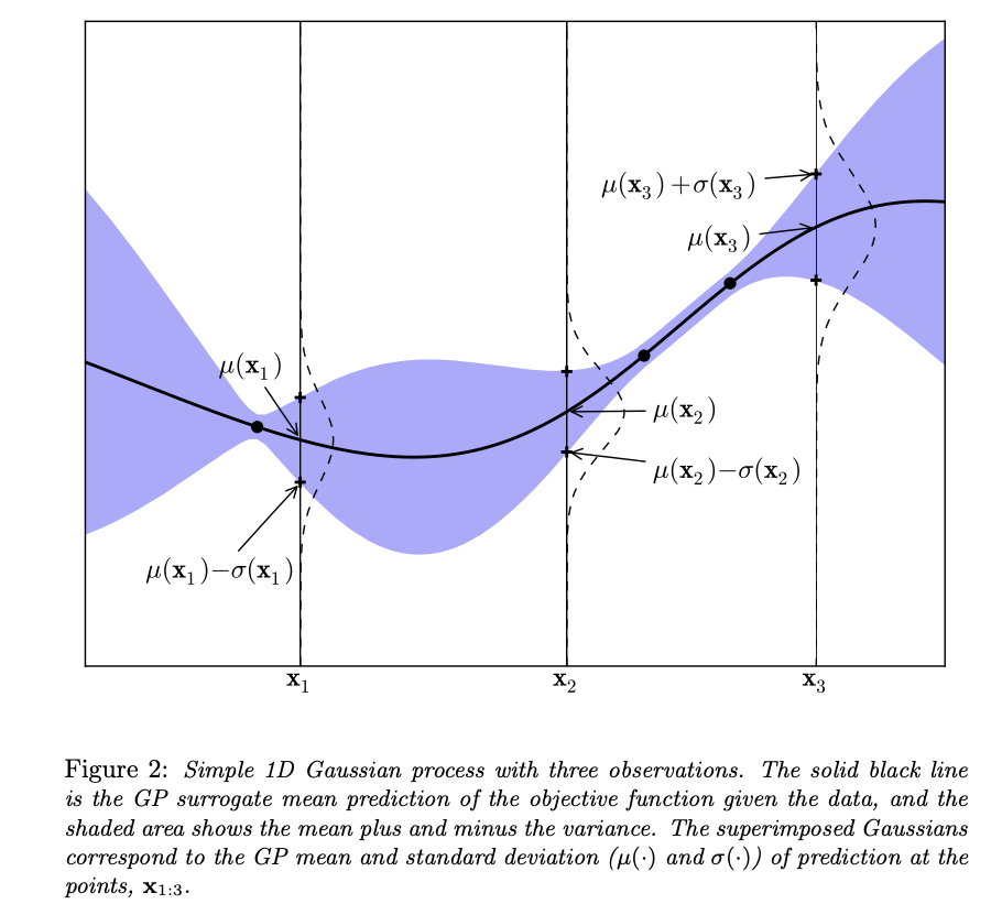
\[\begin{equation} \begin{aligned} \mu_n(x) &= \mu(x) + K(x, \mathbf{x})^\top K(\mathbf{x}, \mathbf{x})^{-1}\big(\mathbf{y} - \mu(x)\big)\\ \sigma_n^2(x) &= k(x, x) - K(x, \mathbf{x})^\top K(\mathbf{x}, \mathbf{x})^{-1}K(\mathbf{x}, x) \end{aligned} \end{equation}\]Therefore, given a prior Gaussian distribution over \(n\) data point \(\mathbf{x} = \{x_i\}_{i=1}^n\), the posterior mean \(\hat\mu(x)\) and variance \(\hat v(x)\) at any arbitrary \(x\) can be calculated by \((5)\). The standard deviation \(\hat\sigma(x) = \sqrt{\hat v(x)}\), the prior \(95\%\) credible interval at \(x\) is within the area \(\big(\hat\mu(x) \pm 1.96 \hat\sigma(x)\big)\):
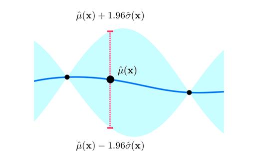
The surrogate model with 95% credible interval at point
Although we have modeled \(f\) at only a finite number of points, the same approach can be used when modeling \(f\) over a continuous domain \(A\). Formally, a Gaussian process with mean function \(\mu\) and kernel \(K\) is a posterior distribution over the function \(f\) with the property that, for any given collection of points \(\mathbf{x}\), the marginal probability distribution on \(f(x)\) is given by \((3)\). Moreover, the arguments that justified \((4)\) still hold when our prior probability distribution on \(f\) is a Gaussian process.
The covariance function \(k(x_i, x_j)\) is also called the “kernel” and expresses the “smoothness” of the process. Kernels typically have the property that points closer in the input space are more strongly correlated, i.e., that if \(\lVert x - x' \rvert < \lVert x - x'' \rvert\) for some norm \(\lVert . \rVert\), then \(k(x, x') > k(x, x'')\). Additionally, kernels are required to be positive semi-definite funciton. A popular choice for the covariance function is the square exponential function, also known as radial basis function (RBF) with the parameter \(\theta\) (to control the width/smoothness of the kernel):
\[\begin{equation} k(x_i, x_j) = \exp\left(-\frac{1}{2\theta^2} \lVert x_i -x_j\rVert ^2 \right) \end{equation}\]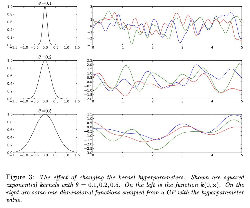
On the other hand, the most common choice for the mean function is a constant value. For convenience, it can be assumed to be the zero function:
\[\mu(x) = 0\]Through the surrogate model, our objective is to update the posterior distribution over the objective function based on new data point \(x^{n+1}\) for optimization. To obtain that new location point, an acquisition function \(\alpha\) is required to guide our search for the optimum. Typically, the acquisitions are defined such that high acquisition corresponds to the potentially high value of the objective function, whether because the prediction is high, the uncertainty is great, or both. Maximizing the acquisition function is used to select the next observation point \(x^{n+1} = \underset{x \in \mathcal{X}}{\operatorname{\arg \max}}\ \alpha(\mathbb{x}\mid D_n)\).
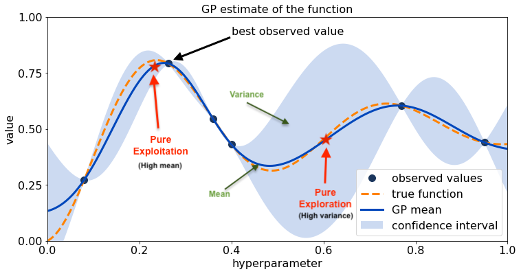
Exploitation (high mean) and exploration (high variance) approaches for acquisition value in sampling the next observed value.
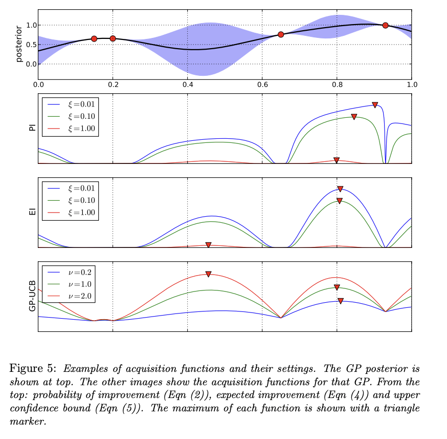
One major challenge of the acquisition function is the trade-off between exploration and exploitation over the surrogate model for the next observed value. The exploitation approach seeks input with high mean (high prediction \(\mu\)), while the exploration seeks input with high variance (high uncertainty \(\sigma\)). Another challenge of the acquisition function is that it must be cheap to evaluate or approximate, “cheap” in relation to the expense of evaluating the black box objective function \(f\). In the following sections, we introduce the most commonly used acquisition functions: Probability of Improvement (PI), Expected Improvement (EI), and Upper Confidence bound (UCB).
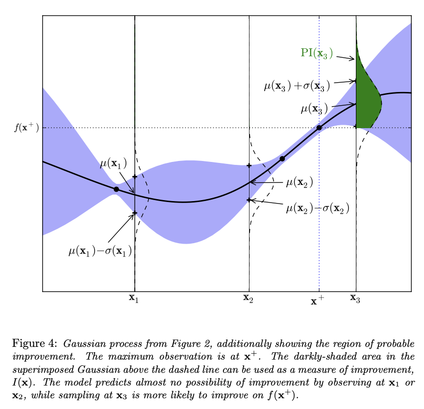
One of the early approach for acquisition function is probability of improvement (PI). Given \(x^+\) is the current optimal point observed: \(x^+ = \underset{x_i \in \mathbf{x}_{1:t}}{\operatorname{\arg \max}} \ f(x_i)\), one early approach for acquisition function is to measure the probability that a point \(x\) leads to an improvement upon \(f(x^+)\) so that:
\[\begin{aligned} \alpha_{PI}(x) &= P\big(f(x) \geq f(x^+)\big)\\ &= \Phi\left(\frac{\mu(x) - f(x^+)}{\sigma(x)}\right) \end{aligned}\]where \(\Phi\) is the c.d.f. of the Gaussian distribution. However, the main drawback of this function is a pure exploitation (heuristic) approach. Specifically, points that have a high probability of being infinitesimally (to an extremely small degree) greater than \(f(x^+)\) will be drawn over points that offer larger gains but less certainty. Therefore, a trade-off parameter \(\epsilon \geq 0\) is added for the trade-off:
\[\begin{equation} \begin{aligned} \alpha_{PI}(x) &= P\big(f(x) \geq f(x^+) + \varepsilon \big)\\ &= \Phi\left(\frac{\mu(x) - f(x^+-\varepsilon )}{\sigma(x)}\right) \end{aligned} \end{equation}\]if \(\varepsilon\) increases, then the acquisition function focuses on exploration rather than exploitation, and vice versa when \(\varepsilon\) decreases.
While seeking the improvement, PI does not measure the amount of improvement. Thus, it cannot always come with the solution for our ultimate quest of finding the global optimum for function \(f\). Therefore, the most plausible way is to calculate how much improvement at each position \(x\), which can be done by:
\[I(x) = \max\big(0, f(x) - f(x^+)\big)\]Thus, \(I(x)\), the improvement at \(x\), is positive when the prediction is higher that the best value known thus far and \(0\) vice versa. Then, the acquisition function is obtained by finding the expected improvement (EI) of \(I(x)\). Similar to PI, an additional parameter \(\varepsilon\) is added for exploration-exploitation trade-off, resulting in:
\[\begin{equation} \begin{aligned} \alpha_{EI}(x) &= \mathbb{E}\big[I(x -\varepsilon)\big]\\ &= \mathbb{E}\big[\max\big(0, f(x) - f(x^+)- \varepsilon\big)\big] \end{aligned} \end{equation}\]With Gaussian Process as the surrogate model, the explicit formula of \(\alpha_{EI}(x)\) is:
\[\begin{equation*} \begin{aligned} \alpha_{EI}(x) &= \begin{cases} \big(\mu(x) - f(x^+) - \varepsilon\big) \Phi(Z) + \sigma(x)\phi(Z) & \text{if } \sigma(x) > 0\\ 0 & \text{if } \sigma(x) = 0 \end{cases} \\ \text{where}\quad Z &= \frac{\mu(x) - f(x^+) - \varepsilon}{\sigma(x)} \end{aligned} \end{equation*}\]where \(\Phi(.)\) and \(\phi(.)\) are respectively the c.d.f. and the p.d.f. of the Gaussian distribution. The figure bellow illustrates a typical new point selection with expected improvement.
Another approach for the acquisition function is based on the upper confidence bound (UCB) of the prediction site, based on multi-armed bandit problem. The guiding principle behind this approach is to be optimistic in the face of uncertainty, thus come with a pure exploration approach. Given a random function model, the Gaussian Process UCB acquisition function is obtained by:
\[\begin{equation} \alpha_{GP-UCB}(x) = \mu(x) + \nu\cdot \sigma(x) \end{equation}\]with \(\nu\) is the upper confidence parameter.
Bellow this the example of the three common acquisition functions and their settings to locate the next datapoint \(x_{n+1}\) for the posterior surrogate distribution.
To find the next observation point at which to sample, we still need to maximize the acquisition function \(\alpha\), thus updating the posterior surrogate model to become approximate with black box \(f\). Unlike the objective function \(f\), \(\alpha\) can be cheaply optimized. However, due to the nature of Bayesian Optimization which receives various type of input space, optimizing \(\alpha\) often have the challenge as in non-convex or multi-modal optimization problems. For continuous input space, some approaches for optimization are space partitioning methods (e.g., DIRECT, LOGO) or gradient based methods (local search).
In short, Bayesian Optimization is a probabilistic optimization based on Bayesian inference to find the global optimal for a black-box objective function \(f(.)\). BayesOpt accepts various types of input \(x\) from continuous space, discrete or combinatorial space (sequences, tree, graphs, sets,…), and hybrid space (the mixture of discrete and continuous variables).
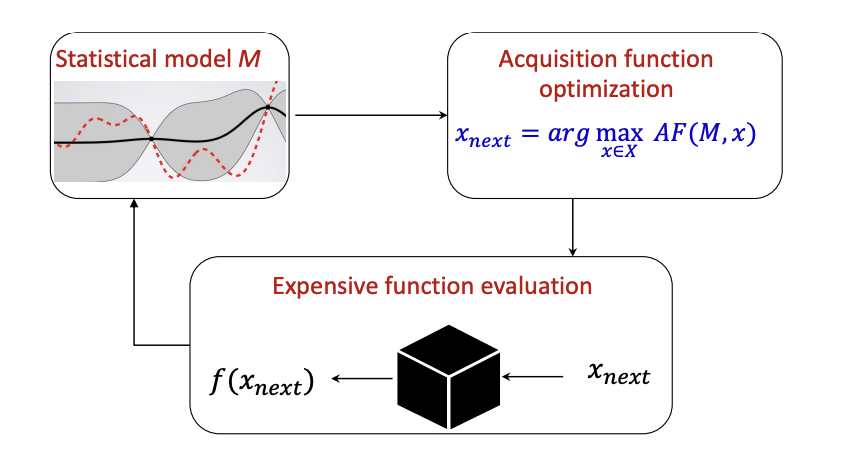
The key idea of Bayesian Optimization is building a surrogate statistical model \(\mathcal{N}\) over the black-box objective function \(f\) and used it to indirectly search for the global optimal point \(x^*\) through a loop. For each step \(n\), an acquisition function \(\alpha\) over \(\mathcal{N}\) is then maximized to sample the next queries sample \(x_{n+1}\) with a far cheaper optimization cost. This new sample \(x_{n+1}\) is then observed by \(f\) to augment the observed data \(\mathcal{D}\) and update \(\mathcal{N}\) to reduce its uncertainty and become approximate with \(f\) by Bayesian Inference \((2)\). Finally, the global optimal \(f(x^*)\) can be found via \(\mathcal{N}\). A more detail algorithm of Bayesian Optimization is presented as follow:
For the statistical surrogate model, the most common choice is Gaussian Process \((3)\) that assumes the uncertainty of the observation \(f(x)\) on any arbitrary point \(x\) follows the normal distribution \(\mathcal{N}(\mu, \sigma)\). Among the acquisition functions, the most common choice is Expected improvement \((8)\) that identifies the next data point \(x_{n+1}\) by maximizing the expectation of the improvement between \(f(x_{n+1})\) and the current maximal observation \(f(x^+)\).
One common practical application for Bayesian Optimization is hyperparameter optimization for training deep learning models, where the deep model can be inferred as a black box, the hyperparameters are hybrid inputs, and the goal is to find the optimal set of hyperparameters so that the deep model can achieve the best performance.