In many real-world or machine-learning problems, we often deal with multiple conflicting tasks at the same time, and each task has its own criteria. Let us visit an example from an economy game theory perspective: Assume we have \(n\) brokers competing for some stocks, and each broker has their own goal and agenda, such as when to buy and when to wait. What we want is to support every body to reach their goal as close as possible, but as the total stocks are limited and cannot fulfill all buyers’ goal, we have to make a compromise to make everyone is happy with their asset so no one should be favored than the others. Of course, there will be multiple solutions for this, and our objective is to find this set of solutions. That is the overall setting of multi-objective optimization.
Basically, multi-objective optimization (MOO) is the problem that the optimal decisions need to be taken in the presence of trade-offs between two or more conflicting objectives. In MOO, the set of optimal solutions is called Pareto Front, in which each solution on the front represents the different trade-off between objectives. A point is Pareto solution if it cannot be improved in any of the objectives without degrading some other objectives.
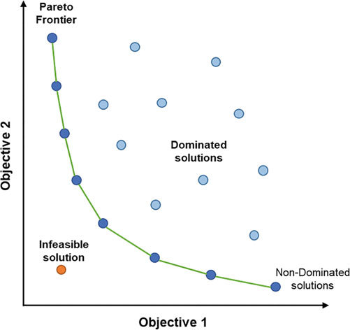
Two-objective optimization with the Pareto Front
Mathematically, MOO is the optimization problem where we have to solve multiple correlated objectives simultaneously:
\[\begin{equation} \begin{aligned} \bm x^* &= \underset{x}{\argmin} \bm f(x)\\ \bm f(x) &=\{f_1(x), \ f_2(x),\cdots, \ f_m(x) \} \end{aligned} \end{equation}\]Where \(m\) is the number of objective functions, \(f_j(x): \mathcal X \rightarrow \mathbb R^m\) is the \(i\)-th objective functions and \(x \in \mathcal X \subset \mathbb R^n\) is the \(n\)-dim solution that need to be optimized.
Based on formula \((1)\), we have some following definitions for the multi-objective optimization problem:
The figure bellows [1] illustrates the examples of Pareto solutions, weakly Pareto solutions, and dominated Solutions. The Pareto solutions are also weakly Pareto optimal. The weakly Pareto optimal but not Pareto optimal solutions (e.g. purple points in Figure a) are dominated but not strictly dominated by at least one Pareto solution (e.g. red points). The weakly Pareto front is the collection of all weakly Pareto optimal solutions \(P_{weak}\) in the objective space. The Pareto front is the collection of all Pareto optimal solutions \(P\) in the objective space.
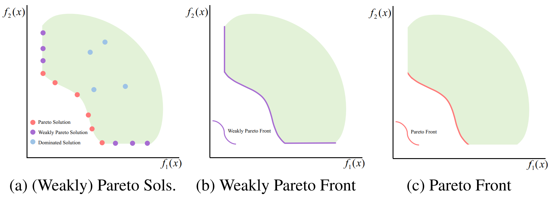
Illustration of the Pareto front on two-objective optimization task
The objective of the MOO problem is to learn the set of Pareto solutions that can approximate the truth Pareto front as close as possible. As the truth Pareto front can be infinite, we need to obtain a finite set of learned Pareto solutions that is diverse enough to sufficiently represent the entire truth Pareto front.
One of the most important metrics for measuring the quality of obtained set of solutions is the hypervolume indicator (HV). The metric is reliable due to its sensitivity to any type of improvement, i.e., whenever an approximation set \(A\) dominates another approximation set \(B\), HV yields a strictly better quality value for the former set than for the latter set. Therefore, any approximation set \(A\) attains with the maximally possible HV value is guaranteed to contain all optimal Pareto solutions.
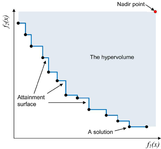
Illustration for Hypervolume indicator
Generally, given a set of solution \(S =\{s_i \subset \mathbb R^m\}\) and a preference point \(r^* \in R^m\), the hypervolume indicator of \(S\) is the measure of the region weakly dominated by \(S\) and bounded above by \(r\) [2]. In particular, we have:
\[\begin{equation} \text{HV}(S) = \bm\Lambda(\{q \in \mathbb R^m \mid \exist s \in S: \ s \bm\prec q \bm\prec r^*\}) \end{equation}\]with \(\bm\Lambda(.)\) denotes the Lebesgue measure on \(\mathbb R^m\), which computes the area of dominated solutions in case of \(m = 2\) and the volume in case of \(m = 3\). The choice for preference point \(r^*\) is often determined depend on the MOO problem, but it usually is the nadir point, i.e., the starting point where all objective functions have the lowest value.
![Hypervolume for the set of solutions $$Y = {y}$$ with $$m = 2$$ and $$m = 3$$ [3]](/assets/blogs/2023-07-12-moo/Untitled%202.png)
Hypervolume with and [3]
A common approach for solving the multi-objective optimization (MOO) problem is transforming multi-objective problem into a single objective optimization (SOO) problem. This can be done with a scalarization functions, parameterized by a preference vector \(\bm \lambda \in \Lambda = \{\bm \lambda \in \mathbb R^m_+ \mid \sum \lambda_i = 1 \}\), to transform MOO to SOO, that is \(\mathfrak s_{\bm\lambda} (f(x)): \mathbb R^m \rightarrow \mathbb R\). Each \(\bm \lambda\) represent a different trade-off over objectives, attaining to a single Pareto solution. Under the scalarization technique, we now consider the MOO problem as single objective optimization. By optimizing \(\mathfrak s_\lambda\), we can obtain a corresponding Pareto solution:
\[\begin{equation} \bm x^*_{\bm\lambda} = \underset{\bm x \in \mathcal X}{\argmin} \ \mathfrak s_{\bm\lambda}(f(x)) \end{equation}\]There are some widely used scalarization functions to tackle the MOO problem:
Weighted sum:
\[\begin{equation} \mathfrak s_{\bm\lambda}(f(x)) = \sum_{i=1}^m \lambda_i f_i(x) \end{equation}\]The advantage of Weighted Sum is in its simplification in computation. However, its main drawback is its inability to find the Pareto solutions in non-convex objective space. Another drawback is the difficulty to set the preference vectors to obtain the Pareto solution in a desired region in the object space.
![Weighted sum scalarization with different weights for convex and non-convex Pareto fronts [4]](/assets/blogs/2023-07-12-moo/Untitled%203.png)
Weighted sum scalarization with different weights for
convex and non-convex Pareto fronts [4]
Weighted exponential sum:
\[\begin{equation} \mathfrak s_{\bm\lambda}(f(x)) = \sum_{i=1}^m \lambda_i [f_i(x)]^p \end{equation}\]While changing \(p\) can help the scalarization function to approximate the Pareto Front, the large value of \(p\) might results in the solutions that is not Pareto optimal.
Weighted Tchebycheff:
\[\begin{equation} \mathfrak s_{\bm\lambda}(f(x)) = \underset{1 \leq i \leq m}{\max}\{\lambda_i \lvert f_i(x) - (z^*_i + \epsilon)\rvert\} \end{equation}\]where \(\bm z^* = (z^*_1, \cdots, z^*_m)\) is the ideal value for the objective functions \(\bm f(x)\), i.e., the lower-bound for minimization problem, and \(\epsilon > 0\) is a small positive scalar, and \((z^*_i + \epsilon)\) is so called the (unachievable) utopia value for the \(i\)-th objective \(f_i(x)\).
![Weighted Tchebycheff scalarization with different weighted for convex and non-convex Pareto fronts [4]](/assets/blogs/2023-07-12-moo/Untitled%204.png)
Weighted Tchebycheff scalarization with different weighted for
convex and non-convex Pareto fronts [4]
By solving the Tchebycheff scalarization function, we can obtain all Pareto solutions \(\bm x \in P\). However, some solutions might be weakly Pareto solution.
HyperNetwork (HN) [3] is a deep neural network \(h(.; \phi)\) that generate weights for a second target network \(f(.; \theta)\). While the target network behaves similar to any usual neural network, i.e. learns to map raw inputs \(x\) to their desire targets \(y\), the hypernetwork receive a set of input \(r\) that contain structure of weight \(\theta\) and generate the weight \(\theta_r\) for \(f(.)\) . While HN is widely used in various domains such as computer vision, continual learning, or federated learning, here we only discuss its application for the MOO task.
![Basic architecture of Hypernetwork [6]](/assets/blogs/2023-07-12-moo/Untitled%205.png)
Basic architecture of Hypernetwork [6]
As the weight \(\theta_r\) produced by a HyperNetwork depend on its input \(r\), we can consider training of the hypernetwork is training a family of target network simultaneously, conditioned on the input \(r\) . Based on that insight, HyperNetwork can be trained to learn the entire Pareto front. Given a single preference vectors \(\bm r \in \mathbb R^m\) that map a set of \(m\)-objective function \(l\) into a single function under a linear scalarization, Pareto HyperNetwork [6] takes \(r\) as inputs to produce the weight \(\theta_r\) via hypernetwork \(h(.)\), then training \(f(.\mid\theta_r)\) to approximate the entire Pareto front. HV Indicator HyperNetwork [7] expand HN framework to learn from multiple preference vectors simultaneously, and maximize the hypervolume (HV) to pushed the learned Pareto front approximated by HN toward the truth Pareto front. Moreover, based on the appropriate preference vector as input, hypernetwork-based approaches can directly generate a corresponding Pareto solution on desired region of the front [8].
![Controlled Pareto solution on selected preference vector with Hypernetwork [8]](/assets/blogs/2023-07-12-moo/Untitled%206.png)
Controlled Pareto solution on selected preference vector with Hypernetwork [8]
In many practical scenarios, we can assume that the set of objectives is unknown and expensive in evaluations, i.e. these objective functions are black-box. Therefore, our target should be learning the Pareto front effectively and efficiently, which is finding the set of optimal solutions as close to the true Pareto front as possible with a limited evaluation budget.
To deal with black-box functions, Bayesian Optimization is an effective choice for optimizing an expensive function with minimal evaluation steps. The main idea for Bayesian optimization is building a statistical surrogate model (Gaussian process) over the objective function and utilizing a simple acquisition function to update the model gradually within a loop and guide the search for optimal value. However, improvements and modifications for Bayesian Optimization mainly for a single objective problem, rather than multiple ones, leaving the potential of multi-objective Bayesian optimization problem (MOBO) opens to exploration.
DGEMO [9] solving the MOBO task by building a surrogate model \(\hat f_i(x)\) and it corresponding acquisition functions for each objective \(f_i(x)\), approximate the Pareto front based on the learned \(\hat f_i(x)\), and selecting the next batch of samples for evaluations. On the other hand, PSL-MOBO [1] combines HyperNetwork with Bayesian Optimization for the MOBO task, by replacing the target network with Gaussian Process models to approximate the target \(m\)-objective functions \(f_i(x)\). Furthermore, Tchebycheff scalarization is applied for mapping multiple objective functions \(f(x)\) into a single one \(g(x\mid\bm \lambda)\) under a preference vector \(\bm \lambda\) for Pareto set learning.
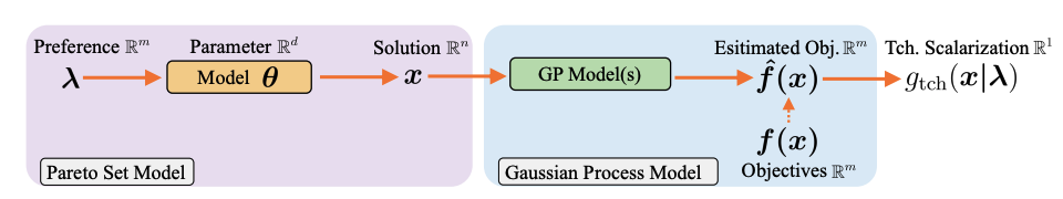
PSL-MOBO for multi-objective Bayesian optimization
In summary, multi-objective optimization is a challenging yet intriguing problem to explore, with the goal is finding the set of optimal solutions (Pareto front) in the presence of trade-offs between multiple conflicting objectives. Minimizing the cost while maximizing comfort when buying a house, minimizing the infrastructural cost while maximizing the durability when building a tower, or maximizing the performance while minimizing the fuel consumption and emission of pollutants when traveling are examples of multi-objective optimization problems with two or three objects. However, there can be more than three objectives in real-world problems.
A typical approach for multi-objective optimization is to convert it to a single objective problem under a scalarization function with a preference vector as weight, representing the trade-off between objectives. Each preference vector comes with a single Pareto solution in the objective space, and our target is to learn a finite set of Pareto solutions diverse enough to represent the whole infinite Pareto front. For such a task, Hypernetwork can be applied to control various preference vectors simultaneously to support the main network learning the Pareto front.
In real scenarios, many of the objectives can be extremely complex and expensive in evaluation, leading to a more challenging problem. To tackle such difficult, Bayesian Optimization can also be utilized for black-box, expensive optimization with minimal optimization steps.